Introduction
Population abundance models are used extensively in ecological studies, and they provide methods of estimation when only site and time replicated counts are available. These models have many possible applications beyond ecology, and can be applied in the study of disease prevalence and detection rates. Yearly counts of reported cases of depression, stratified by Health Service Delivery Area (HSDA), will be used to estimate both the total cases and the case detection rate (CDR) of depression in the Vancouver Coastal Health Authority (VCHA) region from the year 2000 to 2014.
Data, Models and Assumptions
Disease count data is provided by the BC CDC through the Chronic Disease Dashboard. Without this public data, the following analysis would not be possible.
At the time of writing, the Chronic Disease Dashboard is available here. The data tables can be found under the “Tables” heading. We will be looking at “Depression - Age 1+”, with region type “HSDA”.
The counts provided by the BC CDC will be considered partial counts, representative of a larger population of depressed individuals. In this way, we are assuming that there is some unknown probability of detection, or case detection rate, which we will refer to as the CDR.
All model fitting will be done using the R package “unmarked”. I will also be using the “tidyverse” package for data manipulation and visual analysis through “ggplot2”. The packages “knitr” and “kableExtra” will be used to display nicely formatted html tables.
The first model we will fit is a covariate free N Mixture model (developed in the literature by Royle et al. in 2004). This model makes the assumption that the total population of depressed individuals is constant over time (an unrealistic assumption in our case), and that the population is entirely closed to the dynamics of emigration, immigration, new cases, and recovery. This model can be considered a toy model in which we do not expect accurate or even reasonable results, but for which we can provide comparison and contrast with more complicated models. This simple model will be used to illustrate the model fitting and parameter interpretation.
Analysis
For the analysis to follow, we will need these few libraries:
library(unmarked)
library(tidyverse)
library(knitr)
library(kableExtra)
I have downloaded the counts data into a .csv file, and will now load it into R using the following R code. You can see the data.frame is displayed in the table below.
dat <- read.csv("data/bccdc/depression.csv", header = TRUE)

colnames(dat) <- c("Sites", 2000:2014)

kable(dat, "html", caption = "Reported Cases of Depression, VCHA Region") %>%
kable_styling()| Sites | 2000 | 2001 | 2002 | 2003 | 2004 | 2005 | 2006 | 2007 | 2008 | 2009 | 2010 | 2011 | 2012 | 2013 | 2014 |
|---|---|---|---|---|---|---|---|---|---|---|---|---|---|---|---|
| North Shore | 4334 | 4216 | 4055 | 4035 | 3396 | 3563 | 3675 | 3562 | 3446 | 3480 | 3635 | 3632 | 3343 | 3397 | 3073 |
| Richmond | 2375 | 2377 | 2251 | 2126 | 1966 | 1896 | 1856 | 1930 | 1849 | 1834 | 1968 | 1853 | 1724 | 1854 | 1693 |
| Vancouver | 9964 | 9500 | 9123 | 8590 | 7825 | 7571 | 7629 | 7551 | 7346 | 7429 | 7542 | 7590 | 7412 | 7219 | 6904 |
1) Closed Population Model
Our data has three sites (North Shore, Richmond, and Vancouver) which each belong under the VCHA. There are 15 time replications (the years 2000 to 2014). Next we will need to prepare the data for model fitting in “unmarked”. We will be using 1 count = 100 reported cases. This is for computational efficiency, as these models require large computation times which increase with count size. This will reduce our model accuracy, since we will now only be able to report results down to 100’s of cases, however the trade off is that the models will be computationaly feasible on a modern home computer.
# counts
# for computational efficiency, 1 count represented 100 cases
Y <- round(dat[,2:16]/100)
# site covariates
X <- data.frame(Site=as.factor(dat[,1]))
# within site covariates (eg site/sampling occasion specific)
Z <- data.frame(Year=as.factor(rep(2000:2014,3)))

# uframe for closed population/Royle pcount model
uframeC <- unmarkedFramePCount(y=Y,siteCovs=X, obsCovs=Z)
# minimum site population size
Kmin = max(uframeC@y)

kable(as(uframeC, "data.frame"), "html", caption = "unmarkedFramePCount") %>%
kable_styling()| y.1 | y.2 | y.3 | y.4 | y.5 | y.6 | y.7 | y.8 | y.9 | y.10 | y.11 | y.12 | y.13 | y.14 | y.15 | Site | Year.1 | Year.2 | Year.3 | Year.4 | Year.5 | Year.6 | Year.7 | Year.8 | Year.9 | Year.10 | Year.11 | Year.12 | Year.13 | Year.14 | Year.15 |
|---|---|---|---|---|---|---|---|---|---|---|---|---|---|---|---|---|---|---|---|---|---|---|---|---|---|---|---|---|---|---|
| 43 | 42 | 41 | 40 | 34 | 36 | 37 | 36 | 34 | 35 | 36 | 36 | 33 | 34 | 31 | North Shore | 2000 | 2001 | 2002 | 2003 | 2004 | 2005 | 2006 | 2007 | 2008 | 2009 | 2010 | 2011 | 2012 | 2013 | 2014 |
| 24 | 24 | 23 | 21 | 20 | 19 | 19 | 19 | 18 | 18 | 20 | 19 | 17 | 19 | 17 | Richmond | 2000 | 2001 | 2002 | 2003 | 2004 | 2005 | 2006 | 2007 | 2008 | 2009 | 2010 | 2011 | 2012 | 2013 | 2014 |
| 100 | 95 | 91 | 86 | 78 | 76 | 76 | 76 | 73 | 74 | 75 | 76 | 74 | 72 | 69 | Vancouver | 2000 | 2001 | 2002 | 2003 | 2004 | 2005 | 2006 | 2007 | 2008 | 2009 | 2010 | 2011 | 2012 | 2013 | 2014 |
Once the data has been prepared, it is easy to fit the model using the pcount function in “unmarked”. This fits an N Mixture model with covariates specified for abundance and detection rate. We will not specify any covariates for the first model, which corresponds to a constant population size and constant detection rate over sites and time.
The parameter K is an artificial upper bound on the population abundance estimate, and must be chosen such that increasing K does not increase the abundance estimate. To facilitate this choice, we will fit a sequence of models with increasing K, and choose a value of K large enough that no change to the abundance estimate is visible.
It is important to note that K must be larger than the maximum observed count, since the actual population size cannot be smaller than the observed abundance.
# checking for appropriate K
ks <- seq(1*Kmin+1, 2*Kmin,Kmin/50)
Abun <- numeric(0)
for(t in ks) {
  m <- pcount(~1 ~1, uframeC, K=t, se = FALSE, starts=c(5, -0.5))

  r <- ranef(m)
  a <- bup(r)
  Abun <- rbind(Abun, a)
}

# To get abundance we need to multiply by 100 to convert from 1 count to 100 cases.
# We use rowSums to get the total estimate for VCH, rather than the site estimates.
ggplot(data=tibble(ks=ks, Abun=(100*rowSums(Abun))), aes(x=ks, y=Abun)) +
  geom_vline(xintercept = 131, colour="red") +
  geom_line(colour="blue") +
  geom_point() +
  xlab("Upper Bound K") +
  ylab("Abundance Estimate") +
  theme_light() +
  ggtitle("Estimated Abundance vs K")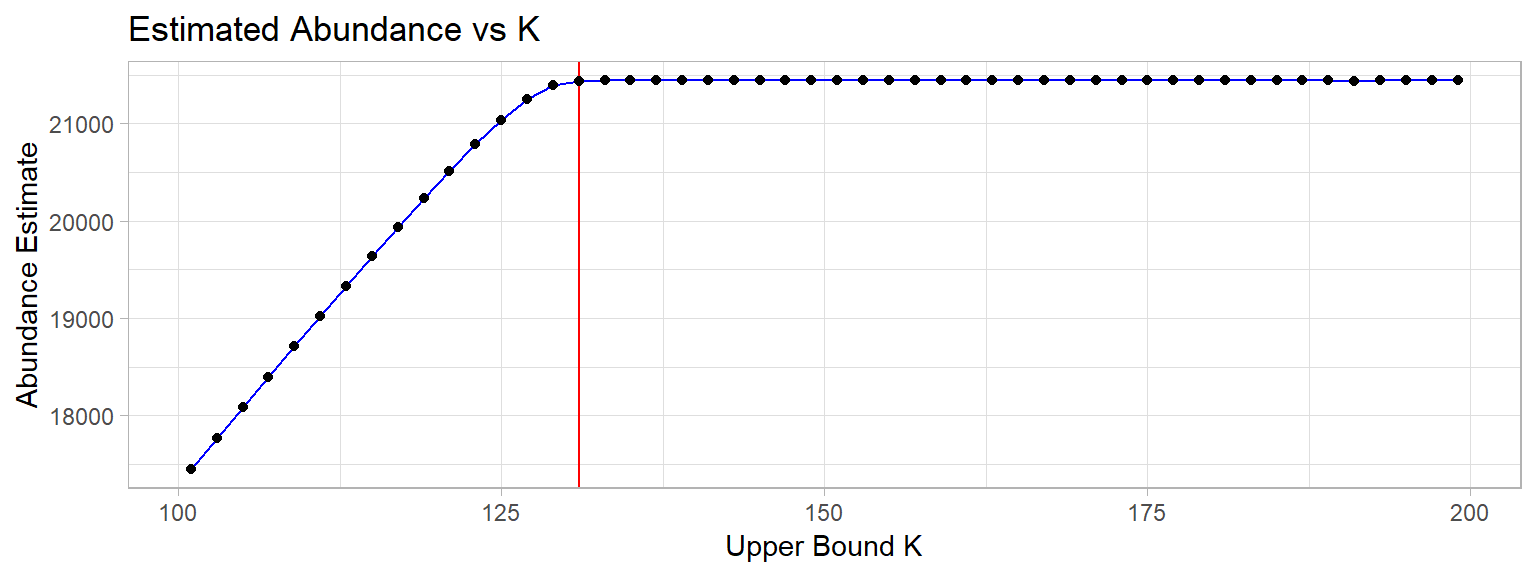
The plot of estimated abundance as a function of increasing K shows that for K>130 (shown by the red vertical line), the estimate is constant. This is a good indication that the maximum likelihood estimates of the parameters have converged. We can choose to use any K value larger than 130, and as such will use K=200 going forwards.
We are now ready to fit the most basic closed population model, and examine the parameter estimates. This will provide a baseline of comparison for the more complicated open population models.
# fit the model
toymodel <- pcount(~1 ~1, uframeC, K=200, se = TRUE, starts=c(5, -0.5))
s_toy <- summary(toymodel)
##
## Call:
## pcount(formula = ~1 ~ 1, data = uframeC, K = 200, starts = c(5,
## -0.5), se = TRUE)
##
## Abundance (log-scale):
## Estimate SE z P(>|z|)
## 4.27 0.094 45.4 0
##
## Detection (logit-scale):
## Estimate SE z P(>|z|)
## 0.545 0.18 3.03 0.00242
##
## AIC: 344.3374
## Number of sites: 3
## optim convergence code: 0
## optim iterations: 28
## Bootstrap iterations: 0det_prob_toy <- plogis(coef(toymodel, type="det"))
det_conf_toy <- confint(toymodel, type="det", level=0.95)
# get model parameter estimates
r_toy <- ranef(toymodel)
a_toy <- 100*bup(r_toy)
# 95% confidence interval (likelihood based)
conf_toy <- 100*confint(r_toy, level=0.95)
df_toy <- data.frame(Site=as.factor(c("North Shore","Richmond","Vancouver")), Abundance_Estimate=round(a_toy), Lower2.5=conf_toy[,1], Upper97.5=conf_toy[,2])
kable(df_toy, "html", caption = "Closed Population Model Abundance Estimates") %>%
kable_styling()| Site | Abundance_Estimate | Lower2.5 | Upper97.5 |
|---|---|---|---|
| North Shore | 5817 | 5500 | 6100 |
| Richmond | 3220 | 3000 | 3400 |
| Vancouver | 12405 | 12000 | 12800 |
ggplot(data=df_toy) +
  geom_errorbar(aes(x=Site, ymin=Lower2.5, ymax=Upper97.5), color="red", width=0.2) +
  geom_point(aes(y = Abundance_Estimate, x=Site ), color="black", size=1.25) +
  ggtitle("Royle Model (~1 ~1)\nAbundance Estimates By Site, with 95% CI") +
  geom_text(aes(x=Site, y=Abundance_Estimate, label=Abundance_Estimate), hjust=-1) +
  geom_text(aes(x=1, y=max(Abundance_Estimate), label=paste0("95% CI for Detection Probability:\n", signif(det_conf_toy[1],2)," < p=",signif(det_prob_toy,2)," < ",signif(det_conf_toy[2],2)))) +
  theme_light()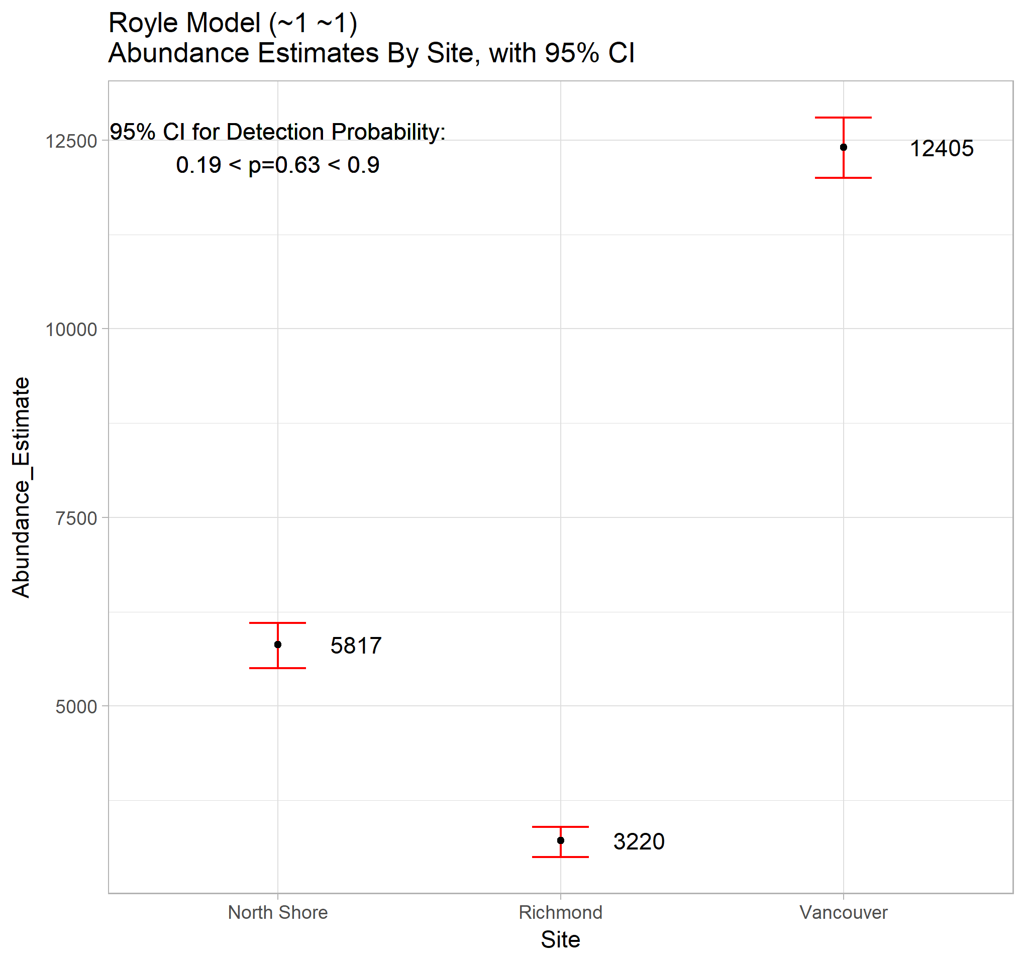
This model predicts a CDR of 0.63, and a total population of depressed individuals of 21400. This leads to a prediction on the unobserved depression cases of 7900. Of course, the model assumptions are not met, so these conclusions are merely for illustration of the methods, and not to be taken seriously.
2) Open Population Model
The open population models are more complicated, allowing for population dynamics. The model will be fit using the function pcountOpen in the “unmarked” package.
The model itself is one where population size for site \(i\) at time \(t+1\) is given by the survival \((S_{it})\) and the population recruitment \((G_{it})\) from time \(t\).
\[ N_{i(t+1)} = S_{it}+G_{it} \] \[ S_{it} \sim Binomial(N_{it}, \omega_{it}) \] \[ G_{it} \sim Poisson(\gamma_{it}) \] These combine with the thinned detection process to give observed counts \(y_{it}\): \[ y_{it} \sim Binomial(N_{it}, p_{it})\]
We will allow initial abundance to vary by site \(\lambda_i=\lambda_{it}\), which seems reasonable as the data suggest significantly different populations at each site. The other parameters will be held constant across time and site so that \(\gamma=\gamma_{it}\), \(\omega=\omega_{it}\), and \(p=p_{it}\). This corresponds to the assumption that the recruitment rate, recovery rate and the detection probability are independent of site and constant over time. The link functions for this model are as follows:
Initial Site Abundance: \[ log(\lambda)=\beta_{0\lambda}+\beta_{1\lambda} * Site \]
Recruitment Rate: \[ log(\gamma)=\beta_{0\gamma} \]
Apparent Survival Rate: \[ logit(\omega)=\beta_{0\omega} \]
Detection Probability: \[ logit(p)=\beta_{0p} \]
# uframe for open population pcountOpen model
uframeO <- unmarkedFramePCO(y=Y, siteCovs=X, yearlySiteCovs=Z, numPrimary = 15)

openmodel <- pcountOpen(lambdaformula = ~Site, gammaformula = ~1, omegaformula = ~1, pformula = ~1, uframeO, K=200, se = TRUE)

# these models take forever to run, so it is good practice to save the model to disk for
# future use, that way you don't need to re-compute from scratch every time
saveRDS(openmodel, here::here("/data/bccdc/openmodel_2018_01_21.RDS"))
openmodel <- readRDS(here::here("/data/bccdc/openmodel_2018_01_21.RDS"))

summary(openmodel)
# get model parameter estimates
r_open <- ranef(openmodel)
a_open <- 100*bup(r_open)
rownames(a_open) <- c("North Shore", "Richmond", "Vancouver")
colnames(a_open) <- 2000:2014
# 95% confidence interval (likelihood based)
conf_open <- 100*confint(r_open, level=0.95)
df_open <- data.frame(Abundance_Estimate=round(as.numeric(a_open),-2), Year=rep(2000:2014, times=rep(3, times=15)), Lower2.5=round(as.numeric(conf_open[,1,]),-2), Upper97.5=round(as.numeric(conf_open[,2,]),-2), Site=as.factor(rep(rownames(a_open), times=15)))
kable(round(a_open, -2), "html", caption = "Open Population Model Abundance Estimates") %>% kable_styling()| 2000 | 2001 | 2002 | 2003 | 2004 | 2005 | 2006 | 2007 | 2008 | 2009 | 2010 | 2011 | 2012 | 2013 | 2014 | |
|---|---|---|---|---|---|---|---|---|---|---|---|---|---|---|---|
| North Shore | 4400 | 4300 | 4200 | 4100 | 3600 | 3600 | 3700 | 3600 | 3500 | 3500 | 3600 | 3600 | 3400 | 3400 | 3200 |
| Richmond | 2400 | 2400 | 2300 | 2200 | 2000 | 1900 | 1900 | 1900 | 1800 | 1800 | 2000 | 1900 | 1800 | 1900 | 1800 |
| Vancouver | 10100 | 9700 | 9300 | 8800 | 8000 | 7700 | 7700 | 7700 | 7400 | 7400 | 7500 | 7600 | 7500 | 7300 | 7000 |
This model predicts a CDR of 0.986, which intuitively seems too large. Reasons for this could be our lack of covariates (both Site and Time based) for the detection probability. Essentially we have assumed that detection probability is constant over time and sites, which is probably not the case. If this article was more than an exploration of the data and the “unmarked” package, we would fit many more models and select those with best performance.
Of course, data are easier to understand when they are presented graphically rather than as tables. So let’s display the results using ggplot2.
# total abundance and 95% confidence intervals by year
df_open_tot <- df_open %>% group_by(Year) %>% summarise(
  Nhat=sum(Abundance_Estimate),
  Lower2.5=sum(Abundance_Estimate)-sum((Abundance_Estimate-Lower2.5)^2)^(0.5),
  Upper97.5=sum(Abundance_Estimate)+sum((Abundance_Estimate-Upper97.5)^2)^(0.5))

# ggplot to display total abundance estimate over time
ggp_open_tot <- ggplot(data=df_open_tot) +
  geom_errorbar(aes(x=Year, ymin=Lower2.5, ymax=Upper97.5), color="red", width=0.2) +
  geom_point(aes(y = Nhat, x=Year), color="black", size=1.25) +
  ggtitle("Open Pop Model (~Site ~1 ~1 ~1)\nAbundance Estimates with 95% CI") +
  geom_text(aes(x=Year, y=Nhat, label=Nhat), vjust=-1) +
  xlab(label = "Year") +
  ylab(label = "Total Estimated Depressed Individuals") +
  scale_x_continuous(breaks=seq(2000,2014,2)) +
  scale_y_continuous(breaks=seq(12000,18000,1000)) +
  theme_light()
ggp_open_tot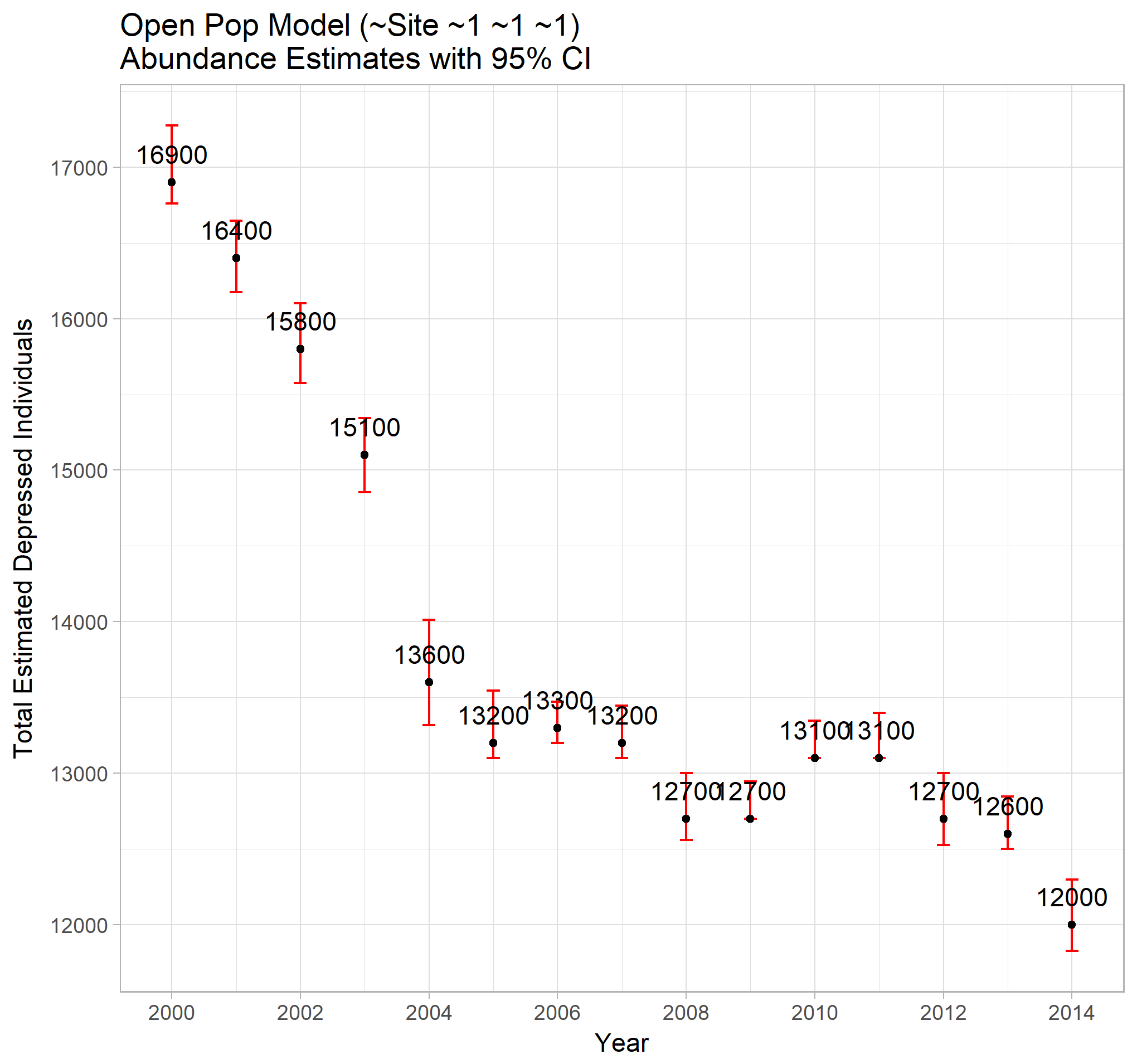
# ggplot to display site abundance estimates
ggp_open_sites <- ggplot(data=df_open) +
  geom_errorbar(aes(x=Year, ymin=Lower2.5, ymax=Upper97.5), color="red", width=0.2) +
  geom_point(aes(y = Abundance_Estimate, x=Year), color="black", size=1.25) +
  ggtitle("Open Pop Model (~Site ~1 ~1 ~1)\nAbundance Estimates with 95% CI") +
  geom_text(aes(x=Year, y=Abundance_Estimate, label=Abundance_Estimate), vjust=-0.6) +
  xlab(label = "Year") +
  ylab(label = "Estimated Depressed Individuals") +
  scale_x_continuous(breaks=seq(2000,2014,2)) +
  facet_grid(Site~., scales = "free_y") +
  theme_light()
ggp_open_sites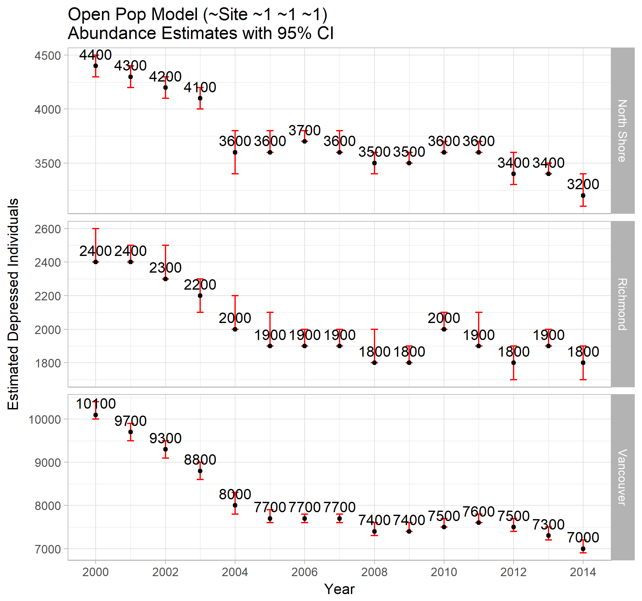
Conclusions
The total abundance estimates indicate that the number of depressed individuals in the VCHA region is declining over time, but at a pace which slowed dramatically between the years of 2004 and 2013. Without data from 2015 onwards, it is impossible to know how the rate has changed since, although the trend since 2011 appears to be decreasing. A time series investigation could provide short term future estimates.
The site specific abundance estimates show a similar decrease in cases across all sites. The Vancouver estimates seem more well behaved than the other two. This could be indicative of systemic changes in those Health Authority regions (perhaps new facilities, new reporting procedures, demographic shifts, region redefinitions, etc). If known, these details could be incorporated into the model for a more accurate set of estimates.
The detection probability was estimated to be 0.986 using the naive but reasonable open population model (compared to the closed population model estimate of 0.63). This value is likely far too high, and we would expect more complex models to do a better job of predicting the detection rate. Access to more covariate information, and modeling of more complex interactions in the link functions, would be ways of potentially improving the estimates.
The fitting of additional models is straightforward, but requires considerable computation time. The comparison of such models can be done through the AIC values (conveniently calculated in the model summary in the “unmarked” package). Lower AIC values would indicate a likelihood preferred model.