Getting bored with the plots you can make using the base R plot? Probably time to spice things up with ggplot!
You can read through this article, or you can watch the tutorial video below (or both!).
Let’s get started. If you haven’t used ggplot before, you will need to install that package by running this either in the R console, or in an R script:
install.packages("ggplot2")To include the library, you just run this:
library(ggplot2)Now that ggplot2 is installed and loaded, we’ll use the data set msleep contained in the ggplot2 package.
sleep <- ggplot2::msleep
head(sleep)
## # A tibble: 6 x 11
## name genus vore order conservation sleep_total sleep_rem sleep_cycle
## <chr> <chr> <chr> <chr> <chr> <dbl> <dbl> <dbl>
## 1 Chee~ Acin~ carni Carn~ lc 12.1 NA NA
## 2 Owl ~ Aotus omni Prim~ <NA> 17 1.8 NA
## 3 Moun~ Aplo~ herbi Rode~ nt 14.4 2.4 NA
## 4 Grea~ Blar~ omni Sori~ lc 14.9 2.3 0.133
## 5 Cow Bos herbi Arti~ domesticated 4 0.7 0.667
## 6 Thre~ Brad~ herbi Pilo~ <NA> 14.4 2.2 0.767
## # ... with 3 more variables: awake <dbl>, brainwt <dbl>, bodywt <dbl>You can see all of the column names (and hence all of the variables we have to play with).
colnames(sleep)## [1] "name" "genus" "vore" "order"
## [5] "conservation" "sleep_total" "sleep_rem" "sleep_cycle"
## [9] "awake" "brainwt" "bodywt"Let’s make a really simple ggplot call to plot “brainwt” versus “sleep_total”:
ggplot(data=sleep) +
  geom_point(aes(x=sleep_total, y=brainwt))
## Warning: Removed 27 rows containing missing values (geom_point).
In the above call there are a few things worth explaining. First, the use of “data=” tells ggplot where to find the data (in this case the column names) which we will be using. Without this, ggplot would not know where “sleep_total” and “brainwt” are located. Second, “geom_point()” is one of many layers that can be added to a ggplot. Layers are added using a “+” between them, as seen in the above ggplot call. You can add as many layers as you’d like to the plot, which allows for very easily customized plots. Finally, “aes()” tells ggplot what aesthetics are mapped to which variables. In the case of “geom_point()”, the two mandatory aesthetics are “x” and “y”. These tell ggplot what the x and y coordinates of each point are. Aesthetics are set equal to column names present in your data in order to map the aesthetic to that variable.
Aesthetics can be used for much more than this however, as they allow you to map colours, shapes, line types, etc. to your variables. As an example, let’s set “color=order” in the aesthetics of the “geom_point()”. While we are at it, let’s also take the log transform of the y aesthetic. This will show off the linear relationship, and make the data easier to look at.
ggplot(data=sleep) +
  geom_point(aes(x=sleep_total, y=log(brainwt), color=order))
## Warning: Removed 27 rows containing missing values (geom_point).
This is showing quite a bit of information, but suppose we want to separate the data into sub plots by group. This is easy to do using “facet_wrap” or “facet_grid”. We will use “facet_wrap” as an example.
ggplot(data=sleep) +
  geom_point(aes(x=sleep_total, y=log(brainwt), color=order)) +
  facet_wrap(~vore)
## Warning: Removed 27 rows containing missing values (geom_point).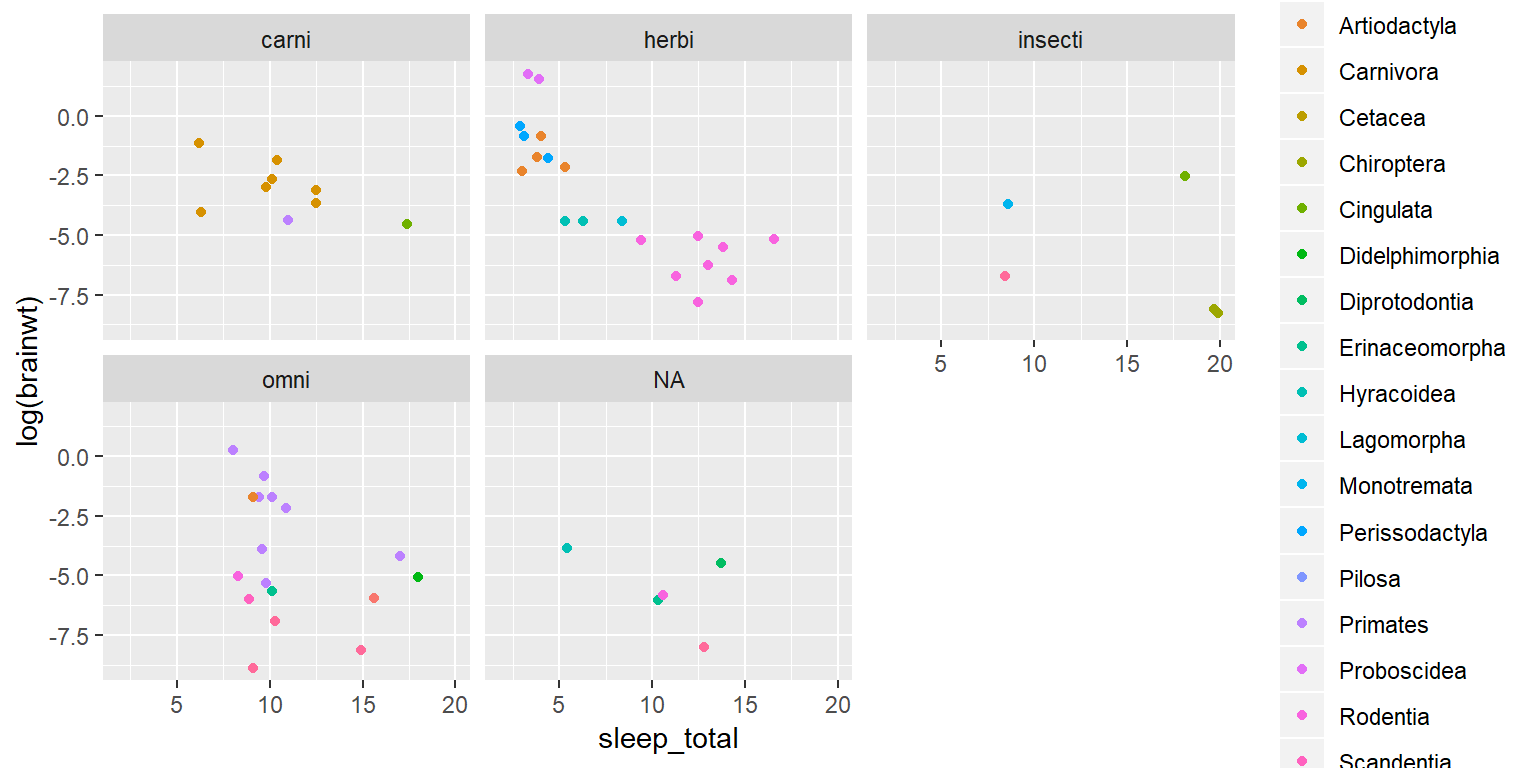
At this point we’ve got a plot, showing some interesting data, using color as an aesthetic and a facet_wrap to separate groups. We’re missing the most basic title, and the labels could use some tidying.
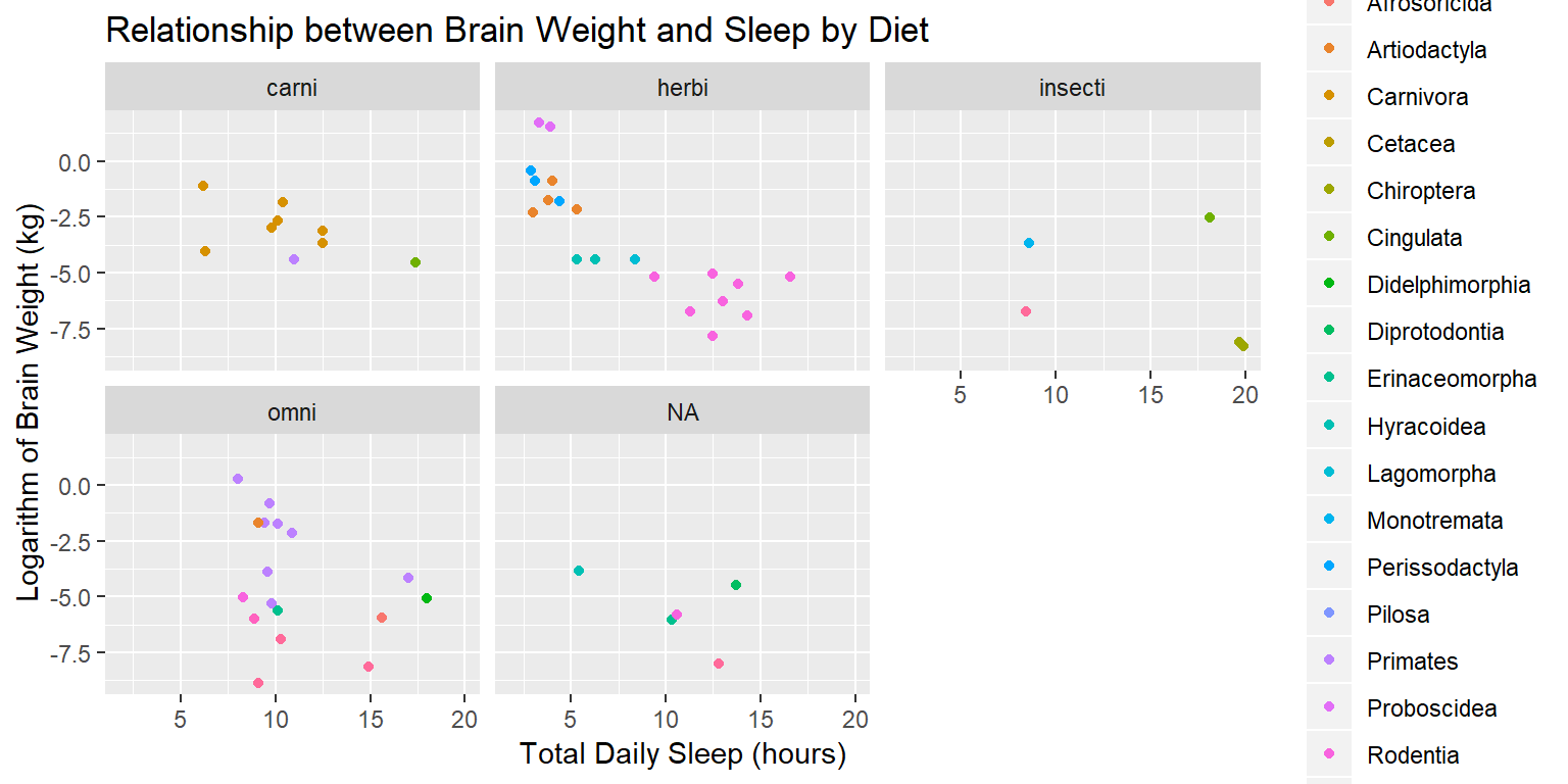
ggplot(data=sleep) +
  geom_point(aes(x=sleep_total, y=log(brainwt), color=order)) +
  facet_wrap(~vore) +
  ylab("Logarithm of Brain Weight (kg)") +
  xlab("Total Daily Sleep (hours)") +
  ggtitle("Relationship between Brain Weight and Sleep by Diet")
## Warning: Removed 27 rows containing missing values (geom_point).