Working on a likelihood function that relies on the Poisson distribution with large mean \(\lambda\), I ran into the problem of underflow! Underflow occurs when a number is too small to be stored in memory, and so it is truncated to be equal to zero. In my case, the probabilities are so small in the tails of the distribution, that the probabilities return as 0 (although there is a non-zero probability in those tails). This may not seem like a problem (close to zero is basically zero right?), however, when you are running an optimizer such as optim, the optimizer can get stuck in the tails of the distribution, where a flat likelihood prevents any updates to the parameters from occuring.
The Problem
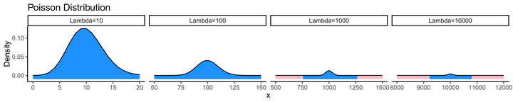
Performing calculations with very small numbers can lead to imprecise results. Often, small numbers will be truncated to zero in computer calculations, and this can have serious implications for scientific research. Let’s take a look at the Poisson distribution for increasing \(\lambda\).
x1 <- 0:20
y1 <- dpois(x = x1, lambda = 10)
x2 <- 50:150
y2 <- dpois(x = x2, lambda = 100)
x3 <- 500:1500
y3 <- dpois(x = x3, lambda = 1000)
x4 <- 8000:12000
y4 <- dpois(x = x4, lambda = 10000)

df <- data.frame(x=c(x1,x2,x3,x4), Density=c(y1,y2,y3,y4), nam=c(rep("Lambda=10",times=length(x1)), rep("Lambda=100",times=length(x2)), rep("Lambda=1000",times=length(x3)), rep("Lambda=10000",times=length(x4))))

ggplot(data=df) + geom_line(aes(x = x, y = Density)) + facet_grid(cols = vars(nam), scales = "free_x") + theme_bw()
Now suppose we are looking at the x values which are 10% different from the mean (x\(=0.9*\lambda\))
# lamda values
lam <- c(10,100,1000,10000, 100000)
# probabilities of observing exactly the quantiles
p <- dpois(x = lam*0.90, lambda = lam)
options(scipen=10)
knitr::kable(x = data.frame(Lambda=lam, Quantile=0.90*lam, Probability=p), digits = 10, align='l')| Lambda | Quantile | Probability |
|---|---|---|
| 10 | 9 | 0.1251100357 |
| 100 | 90 | 0.0250389446 |
| 1000 | 900 | 0.0000751695 |
| 10000 | 9000 | 0.0000000000 |
| 100000 | 90000 | 0.0000000000 |
options(scipen=0)You can see that as \(\lambda\) increases in size, the probability of observations only slightly smaller than the mean are approaching very close to zero. This means that when you are running an optimizer, any observations in the tails of the distribution will return likelihoods of zero.
Libraries
One solution to this problem is to use Arbitrary Precision Arithmetic (APA). Essentially we want to capture the non-zero probabilities even when they are too small for the computer to store as a single number. To accomplish this we will use the library Rmpfr to do APA.
install.packages("Rmpfr")
library(Rmpfr)
Rmpfr Basics
Let’s create an Arbitrary Precision Arithmetic number:
num <- mpfr(5, precBits = 100)
print(num)
## 1 'mpfr' number of precision 100 bits
## [1] 5Okay, that’s not very useful, the number 5 doesn’t need arbitrary precision. Let’s try a very small number:
(paste0("Regular R Arithmetic: ",1/(5^1000)))## [1] "Regular R Arithmetic: 0"num2 <- 1/(num^1000)
(paste0("Arbitrary Precision Arithmetic: ",format(num2)))## [1] "Arbitrary Precision Arithmetic: 1.071508607186267320948425049059e-699"Arbitrary Precision Poisson Distribution
Now we need to create a function that calculates the Poisson density using arbitrary precision.
dpois_apa <- function(x, lambda, prec) {
  # create arbitrary precision arithmetic numbers
  x_apa <- mpfr(x, precBits = prec)
  lambda_apa <- mpfr(lambda, precBits = prec)
  # calculate the density
  dens <- exp(-1*lambda_apa)*lambda_apa^(x_apa)/factorial(x_apa)
  return(dens)
}
Let’s compare this with the regular dpois function:
sum(dpois(x = 0:100, lambda = 900))## [1] 4.368159e-254sum(dpois_apa(x = 0:100, lambda = 900, prec = 100))## 1 'mpfr' number of precision 100 bits
## [1] 4.368158972674260090678233034232e-254Looks good, you can see that they are identical up until the 6th decimal location. Now let’s try with larger lambda (where we have been running into the underflow issue):
sum(dpois(x = 0:1000, lambda = 10000))## [1] 0sum(dpois_apa(x = 0:1000, lambda = 10000, prec = 100))## 1 'mpfr' number of precision 100 bits
## [1] 3.135370556023817217405692086175e-2911Usage With Optim
Rmpfr class objects are not normal numerical objects (you may have noticed that to print the number nicely earlier I had to use print(format(num2)) rather than the usual print(num2)). Because of this we can’t directly use them with the function optim. Luckily the package Rmpfr does contain a single-variable version called optimizeR. That will work for this example, however it won’t be sufficient if you have multiple variables to optimize over.
Here we generate some data, and write two likelihood functions, one with APA, and one without:
# 100 regular observations from a poisson with large lambda,
# plus one outlier at x=100
x <- c(rpois(n = 100, lambda = 10000), 100)

# likelihood function with arbitrary precision arithmetic
L_apa <- function(lambda, obs, prec=100) {
  return(prod(dpois_apa(x = obs, lambda = lambda, prec = prec)))
}

# likelihood function with regular R arithmetic
L <- function(lambda, obs) {
  return(prod(dpois(x = obs, lambda = lambda)))
}
Now we will try to optimize the two likelihoods to estimate \(\lambda\):
# regular optim
optim(par=c(10000), fn = L, method="Brent", lower=0, upper=100000, obs=x)
## $par
## [1] 1e+05
##
## $value
## [1] 0
##
## $counts
## function gradient
## NA NA
##
## $convergence
## [1] 0
##
## $message
## NULL# Rmpfr optimizeR
optimizeR(f = L_apa, lower = 0, upper = 100000, method = "Brent", maximum=TRUE, obs=x)## $maximum
## 1 'mpfr' number of precision 132 bits
## [1] 9912.920792079207931132415194337319594856
##
## $objective
## 1 'mpfr' number of precision 100 bits
## [1] -6.575056585725542566654793125118e-4351
##
## $iter
## [1] 35
##
## $convergence
## [1] TRUE
##
## $estim.prec
## 1 'mpfr' number of precision 132 bits
## [1] 1.527999260997503838156652850858163755956e-16
##
## $method
## [1] "Brent"Interpreting the results above, regular optim was unable to converge, while the optimizeR gives an estimate of \(\hat \lambda=9912.92\dots\); and since we generated the data ourselves, we know that the true value of \(\lambda\) is actually 10000, very close to the estimated value (especially since we biased the data by adding the outlier). We have successfully optimized the likelihood with arbitrary precision arithmetic.