Manifold Regression (part 1)

What is regression?

We will consider regular linear regression (RLR) as an analogy to help understand manifold regression. In RLR, we consider pairs of observations \((x,y)\), with \(x\) the independent variable, and \(y\) the dependent variable. Here, \(x\) and \(y\) are both real numbers. We assume a linear relationship between \(x\) and \(y\), so that \(y=\beta_0 + \beta_1 x\). \(\beta_0\) is the intercept of the straight line formed by plotting \(y\) versus \(x\), while \(\beta_1\) is the slope.

We account for noise/uncertainy/measurement error by adding a random variable \(\epsilon\), drawn independently from a centered normal distribution with variance \(\sigma^2\). Thus the model specification in linear regression is:

\[ \begin{array}{l} y=\beta_0 + \beta_1 x + \epsilon \\ \epsilon \sim N(0,\sigma^2) \end{array} \]

The goal in RLR is then to estimate the two unknown values \(\beta_0\) and \(\beta_1\), from a set of observed pairs \((x_i,y_i)\), with \(i \in 1,2,...,N\).

What is a manifold?

A manifold is a surface embedded in a larger euclidean space, such as how the skin of a ball forms a two dimensional curved surface embedded in a three dimensional space. Similar to how the earth appears locally flat when standing on an open plain, a manifold has the property that anywhere on the manifold, it is possible to “zoom in” arbitrarily close, until the manifold appears flat. For a mathematically rigorous treatment, including defining distance metrics on manifolds, Lee (1997) is a good text.

Symmetric Positive Definite Matrices

A square matrix \(A\) is symmetric if it is equal to its transpose: \(A = A^T\). This means that if \(a_{ij}\) are the entries of \(A\), \(a_{ij} = a_{ji}\). Or that \(A\) is fully specified by its upper triangular elements.

A square matrix \(A\) is positive definite if for every non-zero vector \(b\), the product \(b^T A b\) is greater than zero.

If a matrix \(A\) is symmetric and positive definite, then we say that is it a symmetric positive definite (SPD) matrix. This class of matrices is extremely useful and they show up in real world applications everywhere. A classic example from statistics are covariance matrices, where each entry shows the covariance between two variables (the diagonal entries being the variances of single variables). Covariance matrices are always positive semi-definite (meaning \(b^T A b \ge 0\)), and will be positive definite if the covariance matrix is full rank (meaning that each row is linearly independent of the other rows).

The set of all SPD matrices of size \(n \times n\) form a manifold.

Univariate manifold regression

Fletcher (2011) developed regression methods for a manifold valued response variable \(Y\) against a single real valued regressor \(x\). The regression model has the form:

\[ \begin{array}{l} Y=Exp(P, Exp(V_1 x, E)) \end{array} \]

Where:

• \(P\) is a SPD matrix, called the base point on the manifold
• \(V_1\) is a symmetric matrix, called the coefficient matrix of \(x\)
• \(E\) is a symmetric matrix, called the error matrix

\(Exp(A,B)\) is the exponential map operator, which projects the symmetric matrix \(B\) (which belongs to the tangent space of SPD matrices) onto the space of SPD matrices at the base point \(A\). Therefore, if \(C=Exp(A,B)\), then \(C\) is also an SPD matrix.

Intuitively, the exponential map can be thought of as projecting from the euclidean space onto the embedded manifold. For example, using the Earth as our example manifold, applying the exponential map to a straight line through space (touching the Earth at one point, the base point), would result in a geodesic on the surface of the Earth, passing through the base point.

There is an easy analogy between RLR and manifold regression. The base point \(P\) is like the intercept \(\beta_0\), in that both represent the mean value of the response when the regressor is zero valued. The coefficient matrix \(V_1\) is similar to the slope \(\beta_1\), in that both represent the change in response due to a change in the regressor \(x\).

The two big differences between RLR and manifold regression are

1. the parameters and the response are matrix valued rather than real valued
2. the exponential map, while analogous to addition, has the added benefit of forcing the response variable to exist on the manifold

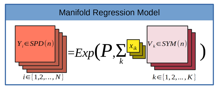
Multivariate manifold regression

Kim et al. (2014) extended the work of Fletcher (2011) for multivariate responses. The framework is the same, but switches from a single regressor/coefficient matrix pair \((x,V_1)\), to several such pairs \(\{(x_1,V_1), (x_2,V_2), ..., (x_k, V_k)\}\). The multivariate manifold regression model has the form

\[ \begin{array}{l} Y=Exp(P, Exp(\sum_{i=1}^{k} V_i x_i, E)) \end{array} \]

Kim et al. (2014) provide algorithms for fitting these multivariate manifold regression models implemented as matlab code. These codes make use of gradient descent to minimize the objective function in searching for the best estimates of the coefficient matrices and the base point. If you use matlab, then you can readily make use of the matlab code provided by Kim et al. (2014) to fit these types of models. However, if you use R, then I have ported the code to an R package MGLMRiem.

Applications

Applications of manifold regression are abundant. Anywhere that your response data takes the form of a covariance matrix, or a correlation matrix, is a good candidate for SPD manifold regression. Many recent applications in health sciences come from medical imaging, including:

• Diffusion Tensor Imaging, see for example Zhu et al. (2009)
• MEG/EEG, see for example Sabbagh et al. (2019)

Other potential applications include fMRI timeseries correlations, brain subnetwork inter and intra covariances, and machine learning algorithms.

For an example showing how to apply these models to your own data, see part 2.

References

Fletcher, T. (2011). Geodesic Regression on Riemannian Manifolds. In Pennec, Xavier, Joshi, Sarang, Nielsen, & Mads (Eds.), Proceedings of the Third International Workshop on Mathematical Foundations of Computational Anatomy—Geometrical and Statistical Methods for Modelling Biological Shape Variability (pp. 75–86). https://hal.inria.fr/inria-00623920

Kim, H. J., Adluru, N., Collins, M. D., Chung, M. K., Bendin, B. B., Johnson, S. C., Davidson, R. J., & Singh, V. (2014). Multivariate General Linear Models (MGLM) on Riemannian Manifolds with Applications to Statistical Analysis of Diffusion Weighted Images. 2014 IEEE Conference on Computer Vision and Pattern Recognition, 2705–2712. https://doi.org/10.1109/CVPR.2014.352

Lee, J. M. (1997). Riemannian manifolds: An introduction to curvature. Springer.

Sabbagh, D., Ablin, P., Varoquaux, G., Gramfort, A., & Engeman, D. A. (2019). Manifold-regression to predict from MEG/EEG brain signals without source modeling. arXiv preprint arXiv:1906.02687.

Zhu, H., Chen, Y., Ibrahim, J. G., Li, Y., Hall, C., & Lin, W. (2009). Intrinsic Regression Models for Positive-Definite Matrices With Applications to Diffusion Tensor Imaging. Journal of the American Statistical Association, 104(487), 1203–1212. JSTOR.