Manifold Regression (part 2)

Getting Data

First, we need a set of data to work from. There are many great fMRI imaging datasets available on the OpenNeuro website. We will use the data of Bhattasali et al. (2020), available here: OpenNeuro.

This data set contains fMRI imaging data for 23 individuals, of which 11 are male and 12 are female. The subjects are aged 18 to 24. Each subject has 372 scans, with \(79\times 95\times 68\) voxels per scan.

We will be using the preprocessed fMRI scans, which have been spatially realigned, smoothed using an isotropic gaussian filter, and transported to MNI space. MNI stands for “Montreal Neurosciences Institute”, and refers in this context to a method of space transformation useful for making comparisons between the brains of different subjects ( whose brains will otherwise have different physical morphologies).

Scans which have not been preprocessed are generally not suitable for this type of analysis, and in general are much more difficult to incorporate into statistical analyses.

Libraries

These are the R libraries we will be using:

library(neurobase)  # for handling .nii files
library(oro.nifti)  # for visualizing .nii data
library(ggplot2)    # for plotting
library(tidyverse)  # for tidy data management
library(abind)      # for appending arrays together

Visualize the Data

The brain imaging data is stored in the .nii format. A very useful R package for reading and visualizing these file formats is neurobase.

Here we are using neurobase for loading the fMRI data for the first subject:

subject1 <- neurobase::readnii(
  "data/fmri/derivatives_sub-18_sub-18_task-alice_bold_preprocessed.nii.gz")

subject1@.Data = subject1@.Data[,,35:37,]
dim(subject1@.Data)

## [1]  79  95   3 372

Notice that we have immediately discarded all but three of the z-layers of the scan. This is to save on memory usage due to the .nii files being very large. If you have a large amount of RAM to work with, then you may not want to do this. After dropping z-layers, we are left with 372 observations of \(79 \times 95 \times 3\) voxels.

Let’s see what this data looks like, note that \(w=90\) selects the 90th time slice/observation:

neurobase::ortho2(subject1, w=90)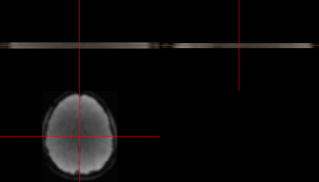

Figure 1: Front, side, and top view of subject 1 at time slice 90.

Above is a view of three slices of the 3D matrix of voxels for subject 1. Each voxel (or 3D pixel) represents the fMRI signal strength for that region of the brain. The first two images are only 3 voxels tall, and this is because we only kept the z-layers for \(z=\) 35, 36 and 37 (which will now be z-layers 1, 2, and 3 respectively). We can also look at all 372 time points in one image:

temp = subject1
temp@.Data = subject1@.Data[,,2,]
oro.nifti::image(temp)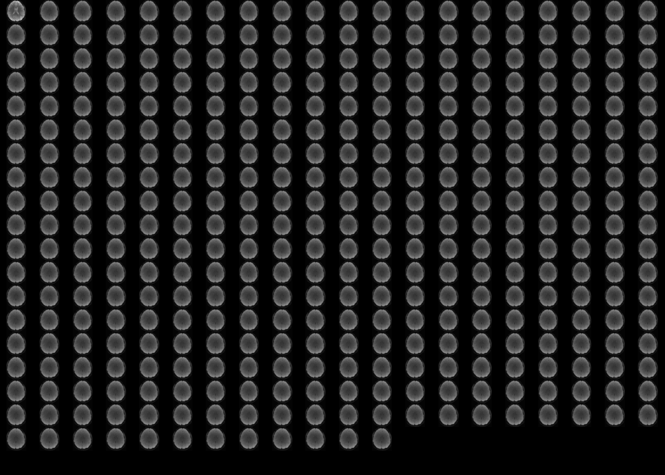

Figure 2: Top view of every time slice for subject 1.

It seems that the first observation is a little bit different than the others:

temp1 = subject1
temp2 = subject1
temp1@.Data = subject1@.Data[,,2,1]
temp2@.Data = subject1@.Data[,,2,2]
oro.nifti::image(temp1)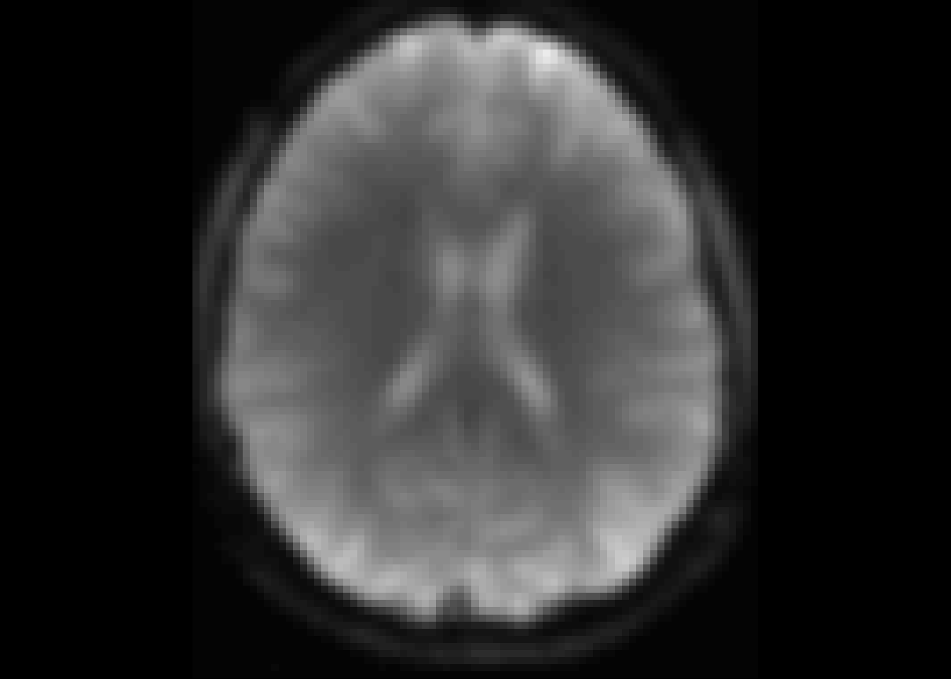

Figure 3: For comparison: time slice 1.

oro.nifti::image(temp2)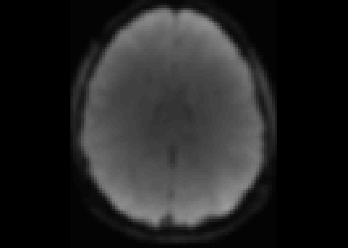

Figure 4: For comparison: time slice 2.

For this reason we will exclude the first time point.

subject1@.Data = subject1@.Data[,,,-1]

Let’s compare to subject 2, where we make the same exclusions, and check for any obvious issues:

subject2 <- neurobase::readnii(
  "data/fmri/derivatives_sub-22_sub-22_task-alice_bold_preprocessed.nii.gz")

subject2@.Data = subject2@.Data[,,35:37,-1]
temp = subject2
temp@.Data = subject2@.Data[,,2,]
oro.nifti::image(temp)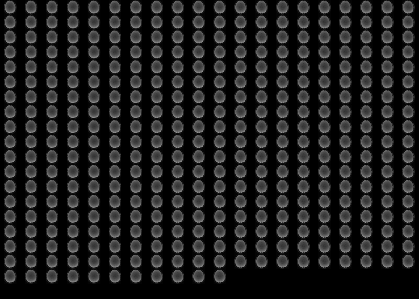

Figure 5: Top view of every time slice for subject 2.

I don’t see any major issues, so we’ll continue on.

Suppose we are interested in a particular brain region. This could come from an image segmentation, brain parcellation, or a brain atlas. In this case we will define our own region of interest (ROI).

ROI = c(32, 49, 1, 2, 2, 2) # x, y, z, l, w, h

The ROI defined above gives us a rectangle in 3D voxel space, where the first three numbers define the starting corner of the rectangle, and the last three numbers define the length, width, and height of the rectangle. In this example, the ROI is a \(2 \times 2 \times 2\) \((l \times w \times h)\) square region with first vertex at \((32,49,1)\).

mask = array(F, dim=dim(subject1@.Data))
mask[(ROI[1]:(ROI[1]+ROI[4]-1)),
     (ROI[2]:(ROI[2]+ROI[5]-1)),
     (ROI[3]:(ROI[3]+ROI[6]-1)),
    ] <- T

s1_mask = subject1
s1_mask@.Data[!mask] <- 0

s1_roi = subject1
s1_roi@.Data = array(subject1@.Data[mask], dim=c(2,2,2,371))

neurobase::ortho2(subject1, s1_mask, w=90, mfrow = c(1,3))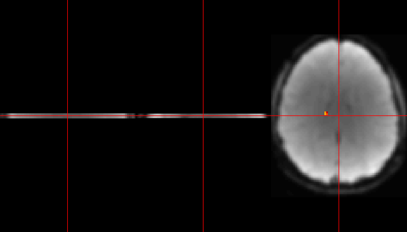

Figure 6: ROI highlighted in red.

neurobase::ortho2(s1_roi, w=90, mfrow = c(1,3))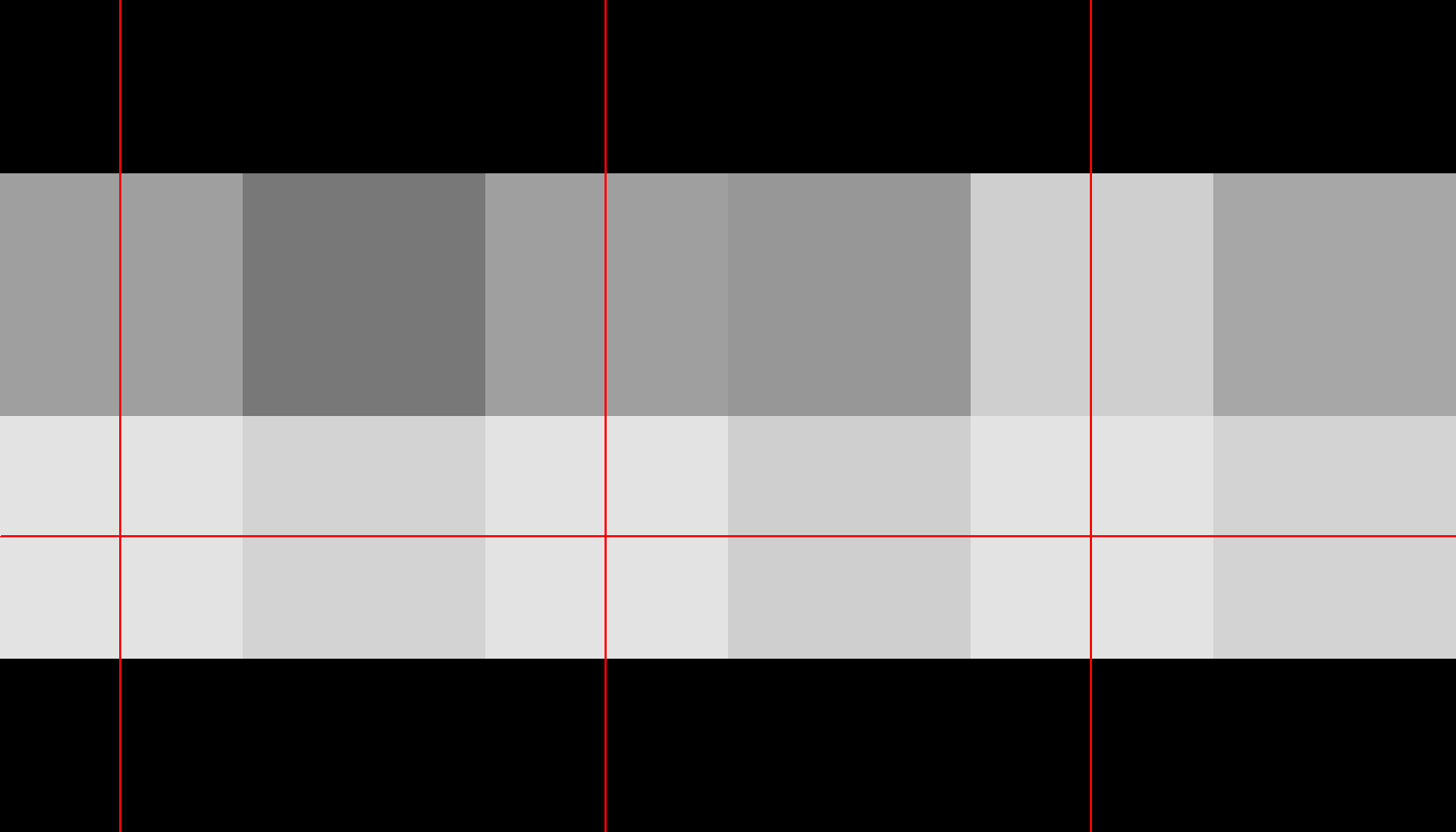

Figure 7: Zoomed in on ROI.

In the first of the above two figures, you see a small red square indicating the location of the ROI. In the second figure, we have zoomed in on all three plots to show only the \(2 \times 2 \times 2\) ROI.

Let \(v_1,v_2,...,v_n\) represent the voxels in the ROI (for this example, \(n=8\)). For a given subject, and a given voxel (for example \(v_1\)), the time series of fMRI measurements looks like this:

timeseries_x = subject1@.Data[32,49,1,]
timeseries_t = 1:dim(subject1@.Data)[4]

plot(x=timeseries_t, y=timeseries_x, type='l', 
     main="fMRI time series: v1",
     xlab="Time Slice",
     ylab="Signal Intensity")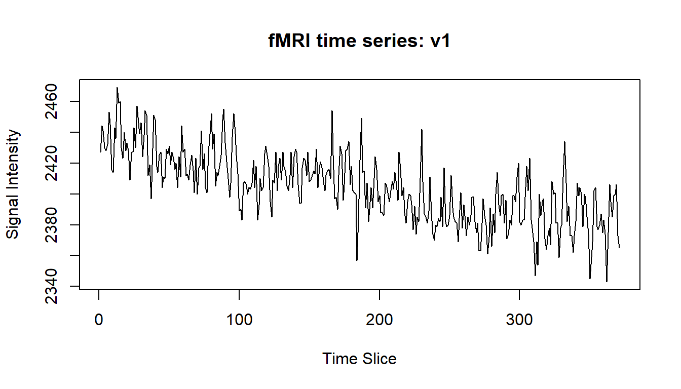

You can see that the time series is non-stationary (the trend in this time series is downwards as time increases). This could be problematic, and one way to address this would be to transform the time series into one which is stationary (using differencing, or subtraction of the mean line). We will leave the time series untouched however, in order to keep things simple.

We would like to be working with symmetric positive definite (SPD) matrices, and so we will use time series covariance matrices. To find the time series covariance matrix for an individual, we calculate:

We can use the symmetric property of the covariance matrix to reduce the number of calculations we need to make. Note that for a correlation matrix, we could also set the diagonal to 1, saving even more computations. This can be relevant in saving computing time for large matrices and large numbers of subjects.

Let’s compute the covariance matrix for each of the 23 subjects:

d = ROI[4]*ROI[5]*ROI[6]

Y = NULL
subject_files = list.files(path="data/fmri")
for(subject in subject_files) {
  
  if(!file.exists(paste0("data/fmri/", subject))) { 
    stop(paste("FILE NOT FOUND:", subject)) 
  }
  
  s_roi = neurobase::readnii(paste0("data/fmri/", subject))
  s_roi@.Data = s_roi@.Data[,,35:37,-1]
  s_roi@.Data = array(s_roi@.Data[mask], dim=c(2,2,2,371))
  
  V = array(0, dim=c(d,371))
  i = 0
  for(x in seq_len(ROI[4])) {
    for(y in seq_len(ROI[5])) {
      for(z in seq_len(ROI[6])) {
        i = i+1
        V[i,] = s_roi@.Data[x,y,z,]
      }
    }
  }
  
  Y1 = array(0, dim=c(d,d,1))
  for(i in seq_len(d)) {
    for(j in seq_len(d)) {
      if(j < i)   { Y1[i,j,1] = Y1[j,i,1] }
      if(j >= i)  { Y1[i,j,1] = cov(V[i,], V[j,]) }
    }
  }
  
  Y = abind::abind(Y,Y1)
}


dim(Y)

## [1]  8  8 23

Notice that \(Y\) is a stack of 23 \(8 \times 8\) matrices. That is 1 covariance matrix each for 23 subjects.

Manifold Regression

We have 23 observations of \(8 \times 8\) SPD matrices. Each of these matrices belongs to either a male or a female subject. We will hypothesise that there is a significant difference from the baseline (\(P\)) between the ROI covariance matrices for male and female subjects, when controlling for age. We will test this hypothesis using manifold regression (Kim et al. 2014), and permutation testing (such as described in Fletcher 2011).

The model we are considering is \(Y = Exp(P, x_1V_1 + x_2V_2)\), where \(Y\) is an SPD matrix, \(P\) is a base point on the manifold (also an SPD matrix), \(V_i\) are symmetric matrices which represent the coefficients of the \(x_i\), \(x_i\) are the covariates. \(x_1\) is an indicator variable which is 0 when subject \(i\) is male, and 1 when female (We could call this covariate genderFemale to be explicit, but to save characters we will call it sex). \(x_2\) is the age in years, standardized by subtracting the mean age and dividing by the standard deviation of age. \(Exp(P,\cdot)\) indicates the exponential map projecting \(\cdot\) onto the SPD manifold at the base point \(P\).

# setup the Male/Female indicator variable and age variable
sex = matrix(c(0,0,1,1,0,0,1,1,0,0,0,0,
                   0,0,1,1,0,1,1,1,1,1,1), nrow=1)
age = matrix(c(22,22,19,21,21,18,19,20,19,21,20,19,
                   19,21,21,22,19,19,20,21,20,18,26), nrow=1)

# note that the X data must be stored in a matrix,
# with each row holding a covariate:
X = rbind(SEX=sex, AGE=(age-mean(age))/sd(age))

We will use the R package MGLMRiem:

remotes::install_github("mrparker909/MGLMRiem")
library(MGLMRiem)

Fitting the model is very easy:

# we are setting the maximum number of iterations to 200,
# this limits how long the gradient descent algorithm will
# take. Also note that the system.time call is only used
# to calculate how long the function runs for, and is in no
# way necessary for fitting the model.
time = system.time({
  mod = MGLMRiem::mglm_spd(X = X, Y = Y, maxiter = 200)
})

The model took 6.78 seconds to converge. These models are CPU intensive to run, and for large problems can be intractable! If you are unsure how long it will take, try setting maxiter to a small number (say 5), and setting enableCheckpoint=TRUE. That way you can both time how long the model fitting will take, and save checkpoints from which you can resume your model fitting.

We can calculate the sums of squares for this model:

Ybar = karcher_mean_spd(Y, niter=200)
SSE=MGLMRiem::SSE_spd(Y, mod$Yhat)
SSE

## [1] 168.8911

SST=MGLMRiem::SST_spd(Y, Ybar)
SST

## [1] 188.4622

SSR=MGLMRiem::SSR_spd(mod$Yhat, Ybar)
SSR

## [1] 18.84356

sprintf("R-squared = %.8f", SSR/SST)

## [1] "R-squared = 0.09998587"

The sums of squared error (SSE) account for about 90% of the total variability (SST). The sums of squares for the regression (SSR) account for around 10% of the variability.

Which is to say, when we account for age and sex, we can explain about 10% of the variation in the observed covariance matrices.

Let’s see how this changes if we only consider age:

mod2 = MGLMRiem::mglm_spd(X = X[2,], Y = Y, maxiter = 200)

SSE2=MGLMRiem::SSE_spd(Y, mod2$Yhat)
SSE2

## [1] 177.8608

SST2=MGLMRiem::SST_spd(Y, Ybar)
SST2

## [1] 188.4622

SSR2=MGLMRiem::SSR_spd(mod2$Yhat, Ybar)
SSR2

## [1] 10.14889

sprintf("R-squared = %.8f", SSR2/SST2)

## [1] "R-squared = 0.05385106"

So both age and sex each account for around 5% of the variability.

However, we should still test whether this small amount of explained variability is significant. We can investigate p-values using a permutation test. Doing this is relatively straight-forward, although exceptionally time consuming (in our case about 3390.00 seconds). We will permute our x-values so that they line up with random y values. We will fit the model to these permuted values, and calculate \(R^2\) values for each of these permutations. We repeat this many times in order to build up a sampling distribution for \(R^2\) under the null hypothesis (the covariates are independent of the observations).

By comparing the distribution of permuted \(R^2\) values to the \(R^2\) value we computed above (\(R^2=\) 0.09998587), we can calculate the probability of observing a more extreme value of \(R^2\) under the null hypothesis. It is important to note that the resolution of this test is dependent on the number of permutations calculated. If you want to test p-values around 0.01, then you need more than 100 permutations. For p-values around 0.001, you need more than 1000, etc.

r2 = NULL
for(i in 1:500) {
  x_perm   = X[,sample(1:length(sex))]
  mod_perm = MGLMRiem::mglm_spd(X = x_perm, Y = Y, maxiter = 100)
  
  SSR_perm = MGLMRiem::SSR_spd(mod_perm$Yhat, Ybar)
  r2 = c(r2, SSR_perm/SST)
}

ggplot() + 
  geom_density(data=data.frame(r2=r2), aes(x = r2), fill = "blue", alpha=0.1) +
  geom_vline(data=NULL, aes(xintercept=SSR/SST), colour="red") +
  geom_label(data=NULL, aes(x=0.13, y=10, label=paste0("Permutation p-value = ", 1-mean(r2 < SSR/SST)))) +
  theme_classic() +
  xlab("R2") +
  ylab("Density (500 Permutations)") +
  ggtitle("Permutation Testing")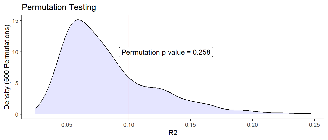

The red line indicates our observed \(R^2\) value. So you can see that even though 10% of the variability could be explained by the model, our results are not statistically significant. Is this surprising?

Not really, the effect size is small, and so we would need a reasonably large sample size to have any certainty in the results. In our case, we are fitting 2 covariates (plus one base point) using only 23 observations. Thus, unless the effect size was quite large, we would not expect to find any statistically significant covariate effects.

To investigate further, we would need a larger sample size. It would also be beneficial to include more covariates which might have an impact on brain connectivity (such as education level, socio-economic status, race, and genetic factors).

I hope this will help you with applying Manifold Regression to your own research problems.

References

Bhattasali, S., Brennan, J. R, Luh, W. M., Franzluebbers, B., & Hale, J. T. (2020). The Alice Datasets: fMRI & EEG Observations of Natural Language Comprehension. In Proceedings of the Twelfth International Conference on Language Resources and Evaluation (LREC 2020)

Fletcher, T. (2011). Geodesic Regression on Riemannian Manifolds. In Pennec, Xavier, Joshi, Sarang, Nielsen, & Mads (Eds.), Proceedings of the Third International Workshop on Mathematical Foundations of Computational Anatomy—Geometrical and Statistical Methods for Modelling Biological Shape Variability (pp. 75–86). https://hal.inria.fr/inria-00623920

Kim, H. J., Adluru, N., Collins, M. D., Chung, M. K., Bendin, B. B., Johnson, S. C., Davidson, R. J., & Singh, V. (2014). Multivariate General Linear Models (MGLM) on Riemannian Manifolds with Applications to Statistical Analysis of Diffusion Weighted Images. 2014 IEEE Conference on Computer Vision and Pattern Recognition, 2705–2712. https://doi.org/10.1109/CVPR.2014.352

University of Zurich. (2018, July 10). Every person has a unique brain anatomy. ScienceDaily. Retrieved April 2, 2020 from www.sciencedaily.com/releases/2018/07/180710104631.htm