optimizeAPA is an R package which allows for multi-parameter optimization. That means you can use it to find the maximum (or the minimum) value of a function with many input values. What makes optimizeAPA unique? It works with arbitrary precision arithmetic.
Why use optimizeAPA?
- 1) works with both APA and NAPA optimization
- 2) works with both single parameter and multi-parameter functions
- 3) save an output file at each iteration
- 4) allows you to keep every value and input visited
- 5) easily plot the convergence path with a single function call
Note: APA stands for “arbitrary precision arithmetic”, while NAPA stands for “non arbitrary precision arithmetic”
APA and NAPA
Using one package for both your APA and NAPA optimization can make troubleshooting and problem solving much easier. You can check the math and logic of your function without arbitrary precision first, and then implement the same function with arbitrary precision. The two functions you will want to use for optimization are optimizeAPA::optim_DFP_NAPA() and optimizeAPA::optim_DFP_APA(). DFP stands for “Davidon-Fletcher-Powell”, and is the only optimization algorithm implemented in the optimizeAPA package (at the time of writing anyways).
Single and Multi-parameter
Other options exist for single parameter optimization (for example Rmpfr::optimizeR()), however, with optimizeAPA you can use the same functions for both single and multi-parameter function optimization. This saves you formatting your data and function multiple times for the various standards and formats employed by different packages.
Save an Output File
Suppose you are not sure if your function will converge within the given number of iterations (the default is maxSteps=100). Then you can save an output file by setting outFile=“output_filename.csv”. This can then be used to give better starting values for a second run of the algorithm.
optimizeAPA::optim_DFP_APA(starts,func,outFile="output_filename.csv",maxSteps=10)Keep Values
By setting keepValues=T in the function call, you can tell the optimization algorithm that you are interested in more than just the last visited function inputs and function value. For example:
optimizeAPA::optim_DFP_APA(starts,func,keepValues = T)There are many reasons why you might want to do this, such as looking for convergence issues, determining better stopping criteria for future simulations (eg: by setting tolerance=10^-3), etc.
optimizeAPA::optim_DFP_APA(starts,func,tolerance=10^-3)Note: the default maximum number of iterations to save when keepValues=T is 100, if you want to keep every value, then set Memory=X, where X is equal to the number you have set for maxSteps.
Plot Convergence
When you set keepValues=T, you can make use of a helper function called optimizeAPA::plotConvergence(). This allows you to view the convergence paths of each input parameter. This can be a very useful visual diagnostic tool.
op <- optimizeAPA::optim_DFP_APA(starts,func,keepValues = T)
optimizeAPA::plotConvergence(op)
Rmpfr
I have covered the R package Rmpfr previously, and you may want to read up on the package if you are interested in writing your own functions to optimize. I will give you a few examples here, which you should be able to modify for your own needs.
Install optimizeAPA
optimizeAPA is available on github, and can be installed using the remotes package:
remotes::install_github("mrparker909/optimizeAPA")Examples
For the folowing examples, we will use these libraries:
library(ggplot2)     # for 2d plots
library(optimizeAPA) # for functional optimization
library(rgl)         # for interactive 3d plots
Single Parameter Function
First, let’s define a regular function F1 to optimize:
F1 <- function(par) {
  (1+par) * sin(2*(par-3)*pi) * exp(-(par-3)^4)
}
Let’s plot the function, so we have some idea of what we’re looking at:
x    = seq(0,6,0.01)
y    = sapply(X=x, FUN=F1)
dat1 = data.frame(x=x,y=y)

ggplot(data=dat1, aes(x=x,y=y)) +
  geom_line() +
  ggtitle("Plot of F1(x)") +
  ylab("F1") +
  theme_classic()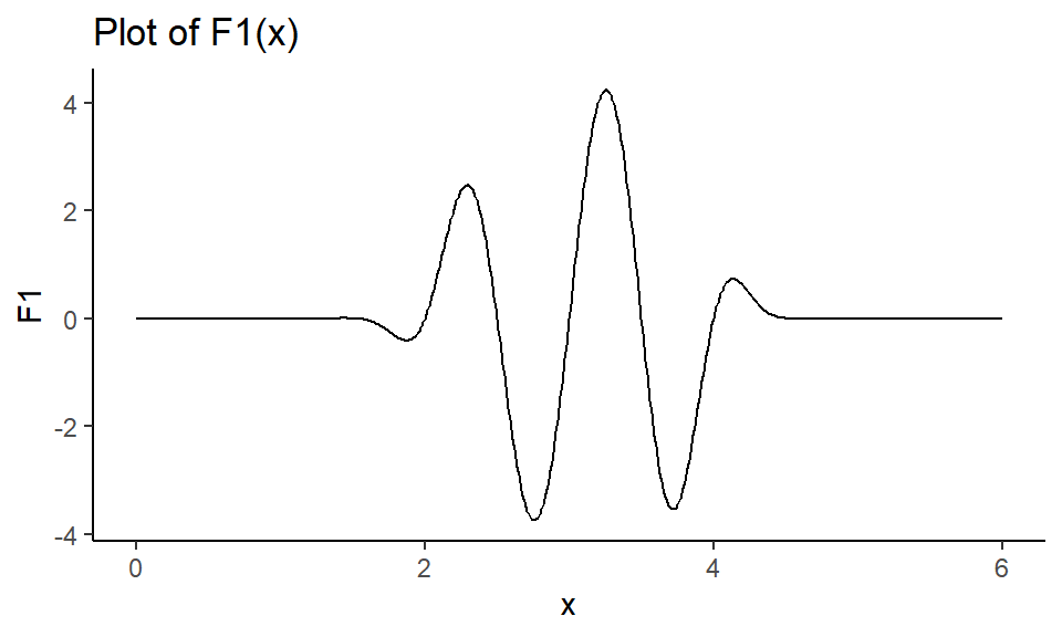
Figure 1: Plot of single parameter function.
We want to find the maximum value \(F_0\) of the function F1, and we want to know what input value \(x_0\) gives us that maximum value. Since the algorithm searches for the minimum, we will input \(-F1\) to find the maximum.
Notice from Figure 1 that the maximum is somewhere between \(x=3\) and \(x=4\), so let’s set \(x=3.5\) as our starting value.
First, the NAPA version:
F1neg = function(par) { -1*F1(par) }
op1 <- optimizeAPA::optim_DFP_NAPA(starts=3.5,
                                   func = F1neg,
                                   keepValues = T,
                                   tolerance=10^-3)
Let’s look at the path to convergence:
optimizeAPA::plotConvergence(op1, flip_axes=T)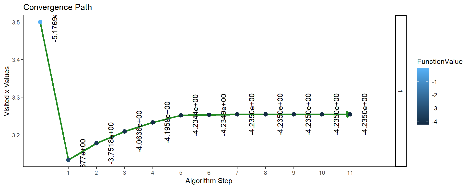
Figure 2: Plot of convergence for single parameter function F1 (NAPA).
So the maximum value of the function (found after 11 iterations of the algorithm) is \(F_0 = F1(3.2543) = 4.235\).
Now we will do the same thing but using arbitrary precision!
# note that precBits allows you to specify the number
# of bits of precision in the calculation
F2 <- function(par, precBits=53) {
  PI = Rmpfr::Const("pi", precBits)
  (1+par) * sin(2*(par-3)*PI) * exp(-(par-3)^4)
}
Now, the APA optimization:
F2neg = function(par, precBits) { -1*F2(par,precBits) }
op2 <- optimizeAPA::optim_DFP_APA(starts=3.5,
                                  func = F2neg,
                                  keepValues = T,
                                  tolerance=10^-3,
                                  precBits = 64)
Let’s look at the path to convergence:
optimizeAPA::plotConvergence(op2, flip_axes = T)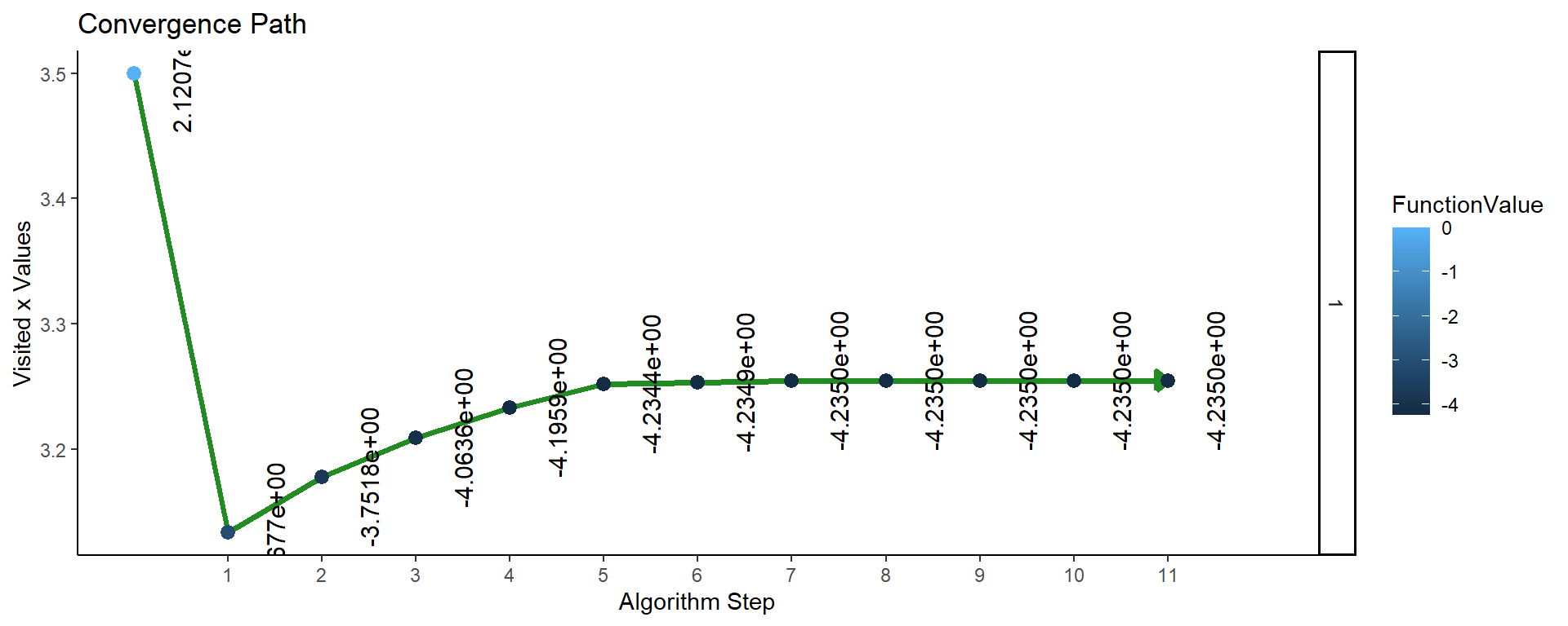
Figure 3: Plot of convergence for single parameter function F2 (APA).
So the convergence plots look the same, but let’s compare the values found by the two algorithms:
knitr::kable(data.frame(algorithm = c("F1: NAPA",   "F2: APA"),
           F_0 = c(Rmpfr::format(-1*op1$f[[1]]),
                   Rmpfr::format(-1*op2$f[[1]])),
           x_0 = c(Rmpfr::format(op1$x[[1]]),
Rmpfr::format(op2$x[[1]]))))| algorithm | F_0 | x_0 |
|---|---|---|
| F1: NAPA | 4.234999 | 3.254283 |
| F2: APA | 4.23499947119854843521 | 3.25428303229783782188 |
You can see that we only have 6 decimal places of precision from the NAPA algorithm (corresponding to 53 bits of precision), whereas the APA algorithm gave us 20 decimal places of precision (corresponding to the 64 bits of precision we chose when we set precBits=64).
Multi-Parameter Function
Functions of a single parameter are not nearly as exciting as functions with many inputs. Let’s augment our previous function F1, so that it takes two inputs.
# now par is a vector of length 2
F3 <- function(par) {
  x = par[1]
  y = par[2]
  (1+x) * sin(2*(x-3)*pi) * exp(-(x-3)^4) *
    (2+y) * sin(2*(y-2)*pi) * exp(-(y-2)^4)
}
# here we define an x,y coordinate grid, and we
# calculate z=F3(x,y) at each point of the grid
x = seq(1,5,length=50)
y = seq(0,4,length=50)
z = outer(x,y,FUN = Vectorize(function(x,y) { F3(par=c(x,y)) }))
par(mai=c(0.4,0,0.1,0))
persp(x,y,z,col="dodgerblue",border="navy",
theta=30,phi=22,shade=0.75,
xaxs="i",yaxs="i",
ltheta=-55,lphi=30)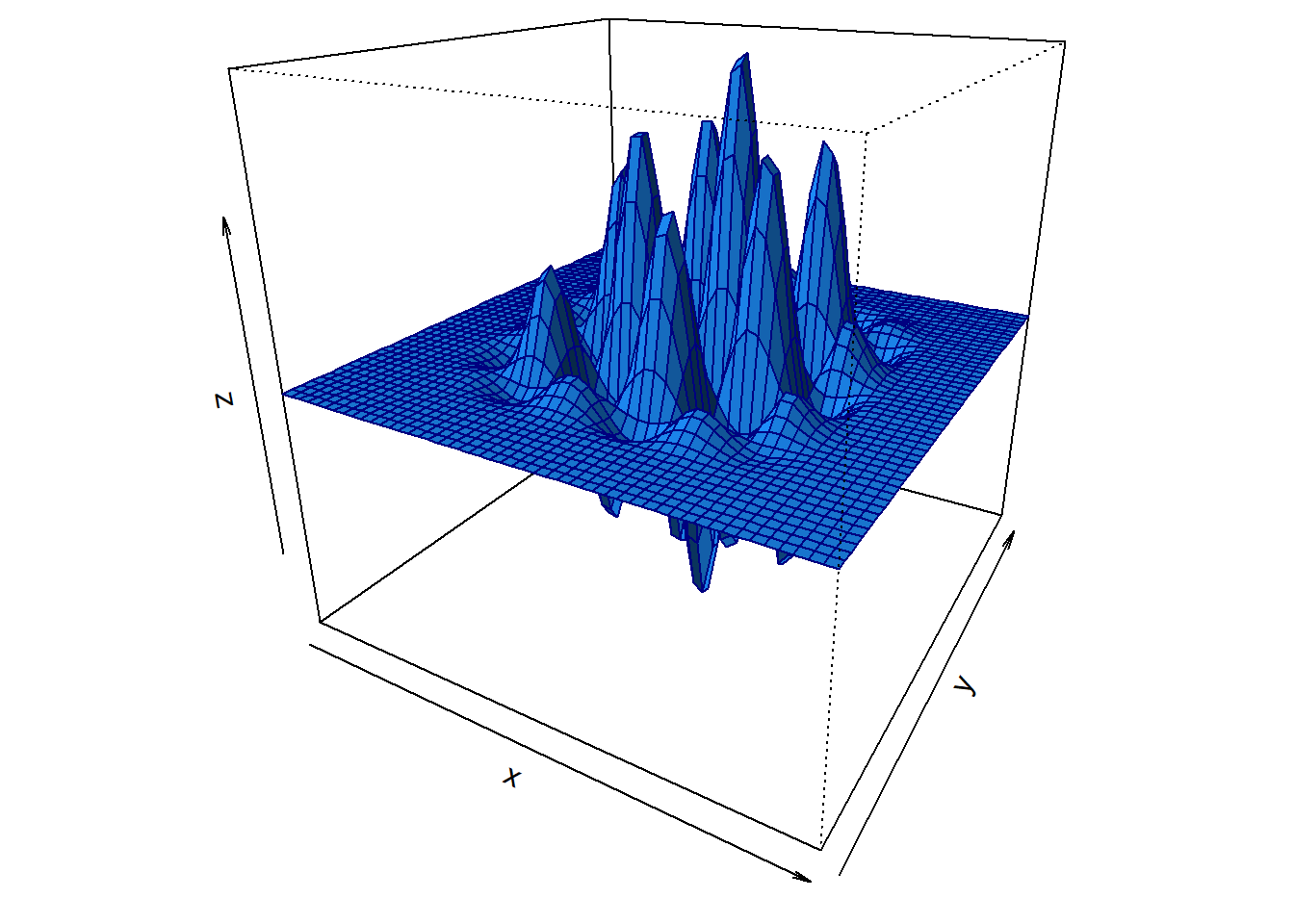
Figure 4: Plot of multi-parameter function.
Now let’s find the maximum value of \(F3\), and the pair of values \(x_0\) and \(y_0\) which maximize the function!
First, we need a good starting point, so let’s use the \(x\) and \(y\) values which gave the largest \(z\):
which(z==max(z), arr.ind = T)## row col
## [1,] 29 29So the starting values are \(x[29], y[29]\) = (3.28571429,2.28571429)
F3neg = function(par) { -1*F3(par) }
op3 <- optimizeAPA::optim_DFP_NAPA(starts=c(x[29],y[29]),
                                   func = F3neg,
                                   keepValues = T,
                                   tolerance=10^-3)
Again we can look at the convergence plot:
# this time we disable the function labels for legibility
# using: labels = F
optimizeAPA::plotConvergence(op3, labels = F, flip_axes = T)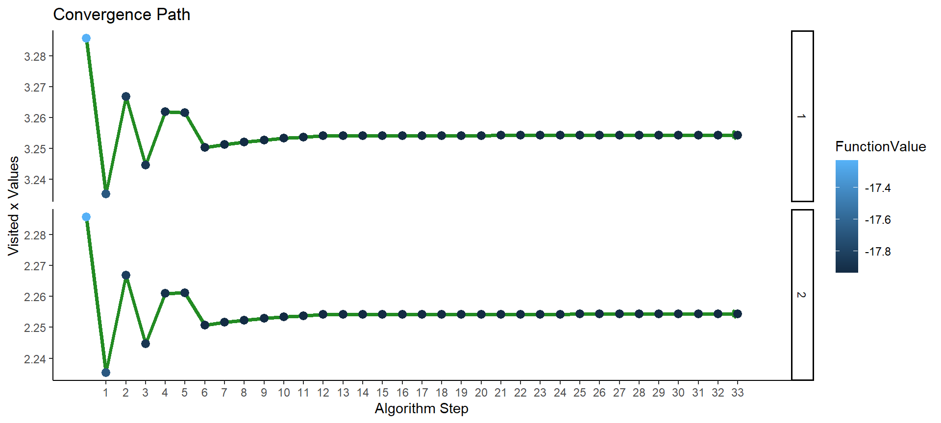
Figure 5: Plot of convergence for multi-parameter function F3 (NAPA).
The algorithm converged after 33 iterations. We can get at the maximum function value and at the values of \(x\) and \(y\) which jointly maximize the function:
-1*op3$f[[1]] # note that we multiply by -1 to undo our previous transformation## [1] 17.93522op3$x[[1]] # note that "x" here denotes c(x,y)## [,1]
## [1,] 3.254288
## [2,] 2.254288The maximum value of \(F3\) is 17.9352205, and that value is attained by \(x=\) 3.2542878, and \(y=\) 2.2542877.
We can also visualize what has happened by plotting the convergence path on the 3D plot of the function:
# here we define an x,y coordinate grid, and we
# calculate z=F3(x,y) at each point of the grid
x = seq(3.23,3.29,length=50)
y = seq(2.23,2.29,length=50)
z = outer(x,y,FUN = Vectorize(function(x,y) { F3(par=c(x,y)) }))

# using rgl
persp3d(x,y,z,col="dodgerblue",border="navy",
        theta=30,phi=22,shade=0.75,
        xaxs="i",yaxs="i",
        ltheta=-55,lphi=30, alpha=0.45)
lines3d(x=unlist(op3$x)[c(T,F)],
        y=unlist(op3$x)[c(F,T)],
        z=-1*unlist(op3$f),
        col="blue", size=5)
points3d(x=unlist(op3$x)[c(T,F)],
         y=unlist(op3$x)[c(F,T)],
         z=-1*unlist(op3$f),
         col="red", size=5)
rgl.postscript(filename = "img/rgl-snapshot.pdf", fmt = "pdf")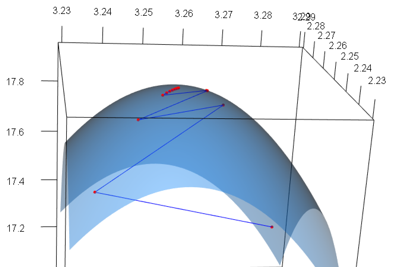
Figure 6: Plot of multi-parameter function (zoomed near maximum). Visited points shown in red, path of convergence traced in blue.
Let’s make \(F3\) APA:
F4 <- function(par, precBits=53) {
  x = par[1]
  y = par[2]
  PI = Rmpfr::Const("pi", precBits)
  (1+x) * sin(2*(x-3)*PI) * exp(-(x-3)^4) *
    (2+y) * sin(2*(y-2)*PI) * exp(-(y-2)^4)
}
F4neg = function(par, precBits) { -1*F4(par, precBits) }
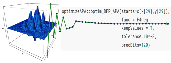
op4 <- optimizeAPA::optim_DFP_APA(starts=c(x[29],y[29]),
func = F4neg,
keepValues = T,
tolerance=10^-3,
precBits=120)This time the convergence plot is slightly different, and the convergence took 38 steps to achieve:
# this time we disable the function labels for legibility
# using: labels = F
optimizeAPA::plotConvergence(op4, labels = F, flip_axes = T)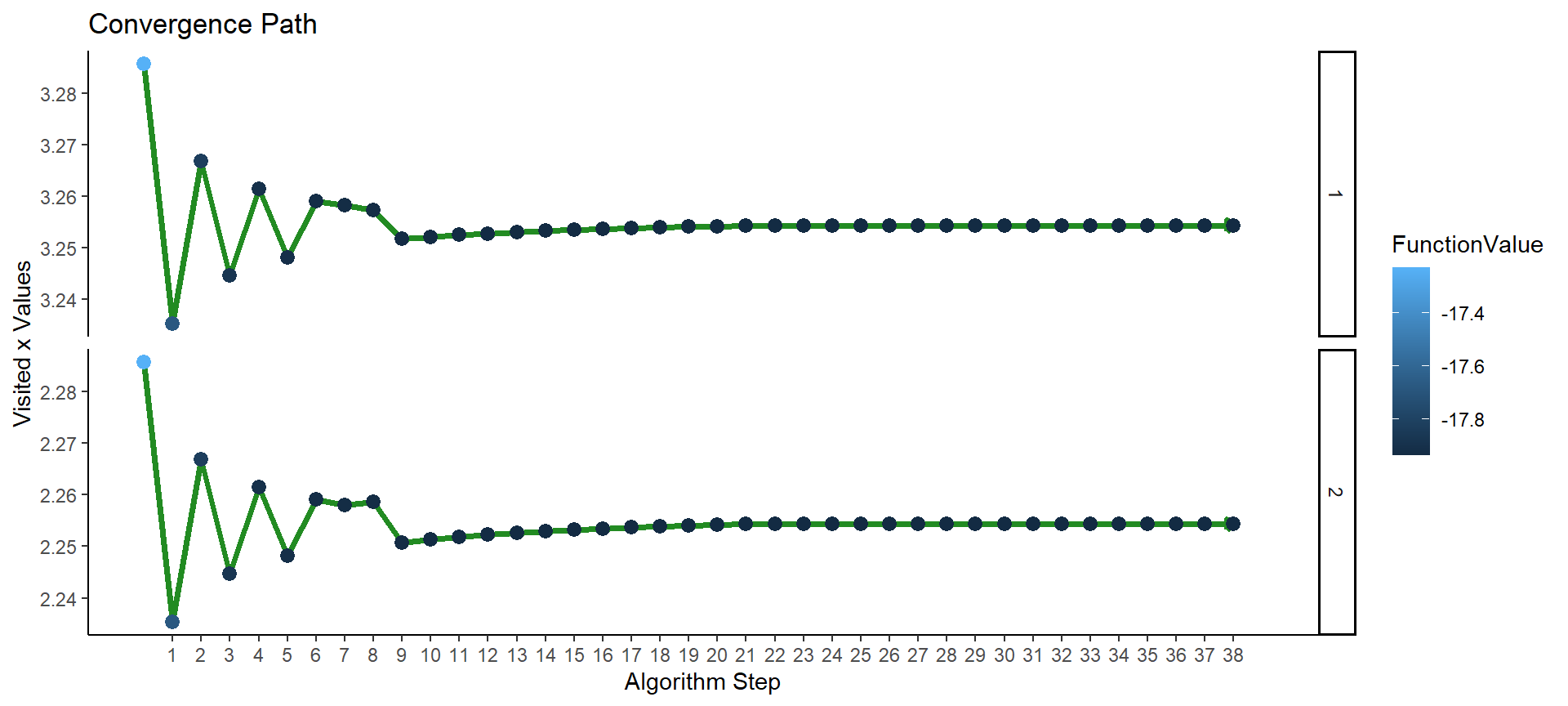
Figure 7: Plot of convergence for multi-parameter function F4 (APA).
knitr::kable(data.frame(algorithm = c("F3: NAPA",   "F4: APA"),
           F_0 = c(Rmpfr::format(-1*op3$f[[1]]),
                   Rmpfr::format(-1*op4$f[[1]])),
           x_0 = c(Rmpfr::format(op3$x[[1]][1]),
                   Rmpfr::format(op4$x[[1]][1])),
           y_0 = c(Rmpfr::format(op3$x[[1]][2]),
Rmpfr::format(op4$x[[1]][2]))))| algorithm | F_0 | x_0 | y_0 |
|---|---|---|---|
| F3: NAPA | 17.93522 | 3.254288 | 2.254288 |
| F4: APA | 17.935220532183663378291420336576143962 | 3.2542876863244057572412360419991646041 | 2.2542879503583251025434494774779739170 |
Of course you can use these methods on functions of many more variables, just use par as a vector to hold each of the parameters to be optimized over.
As a word of caution, changing tolerance is essentially setting the accuracy of the optimization (where as changing precBits is setting the precision). This means that decreasing tolerance can improve the results of the algorithm, but be warned that it likely will also take more iterations to converge. Have a look at the gradient field of the optimization output for some idea of how close to the maximum (or minimum) the algorithm has gotten:
op4$grad[[1]]## 2 'mpfr' numbers of precision 120 bits
## [1] 0.0004730224609375 0.00066280364990234375Note that the closer to zero each of the values in the gradient is, the closer the algorithm is to a local minimum or maximum.
Conclusions
There is a ton more that you can do with optimizeAPA, and the package is still being developed, so expect more in the future. You can have a look at the package README for a few more examples.
References
Davidon, W. (1959). Variable metric method for minimization. Technical Report ANL-5990, 4252678.