Bootstrap Tutorial in R

What is bootstrapping?

The bootstrap essentially uses re-sampling of a set of sample data in order to observe properties of the distribution of the data. For each re-sampling of the data (each “bootstrap sample”), you sample with replacement from the sample data, and compute the statistic of interest on the bootstrap sample (the bootstrap statistic). This provides you with a set of bootstrap statistics from which you can analyze the estimated sampling distribution of the statistic.

Bootstrap Example

Let’s look at a very simple example. Suppose that you have had fifteen people independently measure the length (in meters) of a particular dog named Oscar, and you are interested in the standard deviation of the measurements. It is easy to calculate the estimated standard deviation of the measurements, but how can you estimate the accuracy of the estimated standard deviation?

For the sake of illustration, we know ahead of time that Oscar is 1.15 meters long, and depending on the person who measures him (and how much extra hair they measure on his tail) the standard deviation is 0.05, with the measurement error following a Normal distribution.

set.seed(12345)
oscarL = round(rnorm(n = 15, mean = 1.15, sd = 0.05),3)

# 15 measurements of Oscar's length in meters
oscarL

##  [1] 1.179 1.185 1.145 1.127 1.180 1.059 1.182 1.136 1.136 1.104 1.144 1.241
## [13] 1.169 1.176 1.112

The estimated standard deviation is then:

sd(oscarL)

## [1] 0.04316855

So how do we describe the error associated with the estimated standard deviation? Well, we can increase our effective sample size for our statistic from 1 up to \(B\) by resampling our data \(B\) times (to obtain \(B\) bootstrap estimates for standard deviation). Let’s see what happens when we resample 100, 1000, and 10000 times.

First we define a bootstrap function to make our lives easier:

# Define the function BOOTSTRAP() to do our bootstrapping.
BOOTSTRAP <- function(data, B) {
  # define the statistic to be calculated,
  # in our case it is just the standard deviation
  calc_statistic <- function(sample_data) {
    sd(sample_data)
  }
  
  # here we resample the data, and calculate the bootstrap statistic
  BOOT_STAT <- function() {
    bootstrap_sample = sample(x = data, size = length(data),replace = T)
    calc_statistic(bootstrap_sample)
  }
  
  # here we perform the bootstrap B times
  s = replicate(n = B, expr = BOOT_STAT(), simplify = T)
  return(s)
}

Now we perform the bootstrap:

set.seed(53421) # setting seed for bootstrap reproducibility

resamples = c(1e2, 1e3, 1e4) # B = 100, 1000, 10000

# calculate the bootstrap standard deviations
bootstrap_sd  = lapply(X = resamples, FUN = BOOTSTRAP, data=oscarL)

# calculate the three bootstrap standard deviations of 
# the estimated standard deviation
bootstrap_sdsd = sapply(X = bootstrap_sd, FUN = sd)

# save the results to a data.frame
bootstrap_df = data.frame(
  BootstrapSamples = format(resamples, scientific = F), 
  StandardDeviation = bootstrap_sdsd)

bootstrap_df

##   BootstrapSamples StandardDeviation
## 1              100       0.008288609
## 2             1000       0.008729073
## 3            10000       0.008534525

Since the standard deviation of the estimated standard deviation is not changing too drastically with increasing bootstrap samples, we’ll go with the results from 10000 bootstrap samples. This gives us an estimated standard deviation of 0.0432 \(\pm\) 0.0085. Notice that in this case, the true standard deviation of 0.05 lies within the estimated interval of (0.0346, 0.0517).

A better approach would be to use a confidence interval rather than the standard deviation of the bootstrap estimates. There are many advantages to this approach, and in particular it allows you to specify a confidence level for your bootstrap estimate.

Here is one way you can get at the 95% confidence interval:

bootstrap_sd_CI = lapply(bootstrap_sd, quantile, probs = c(0.025,0.975))
  
bootstrap_df_2 = data.frame(
  BootstrapSamples = format(resamples, scientific = F), 
  CI_lower = unlist(bootstrap_sd_CI)[c(T,F)], 
  CI_upper = unlist(bootstrap_sd_CI)[c(F,T)])

bootstrap_df_2

##   BootstrapSamples   CI_lower   CI_upper
## 1              100 0.02206200 0.05739329
## 2             1000 0.02408351 0.05802511
## 3            10000 0.02404507 0.05769014

This approach gives us an estimated standard deviation of 0.0432, with a 95% confidence interval of (0.0240,0.0577).

It can also be useful to look at the distribution of the bootstrap statistic, as this can illustrate potential problems (such as skewness, holes in the support, etc). This is also not difficult to do:

library(ggplot2)
df_density = data.frame(bootstrapSD = bootstrap_sd[[3]])
df_CI = data.frame(CI = c(round(bootstrap_df_2$CI_lower[3],4),
                          round(bootstrap_df_2$CI_upper[3],4)))
ggplot() + 
  geom_density(data = df_density, 
               aes(x = bootstrapSD)) +
  geom_vline(data = df_CI,
             aes(xintercept = CI), color = "dodger blue") +
  geom_text(data=df_CI, aes(y = 40, x=CI, label=CI)) +
  theme_classic() + 
  xlab("Bootstrap Estimated Standard Deviation") +
  ylab("Density") +
  ggtitle("Bootstrap Sampling Distribution", 
          subtitle = "10,000 bootstrap samples, 95% CI in blue")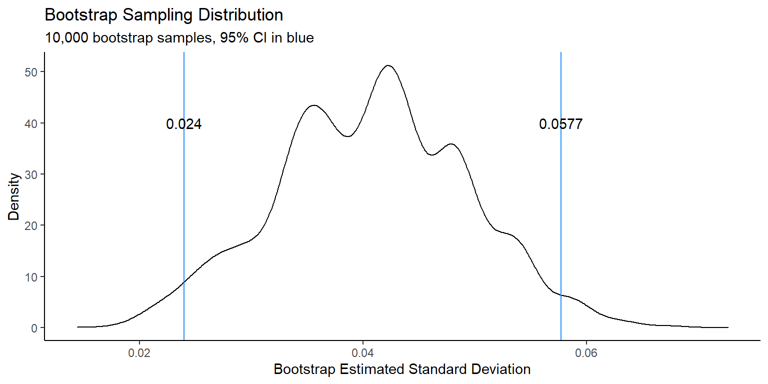

Figure 1: Density plot for 10,000 bootstrap sample statistics with 95% confidence interval.

You can see from the figure that the estimated sampling distribution for the estimated standard deviation has several peaks. This is because we only started with 15 data points. In general, the bootstrap performs better when the initial sample size is larger. However, as you have seen in this example, it can perform quite well even for such a small sample size.

Conclusions

There is a great deal more that can be done with the statistical bootstrap technique, including multivariate bootstrapping, robust bootstrapping, parametric bootstrapping, smoothed bootstrapping, windowed bootstrapping, etc. I hope that this brief introduction will help you with applying the bootstrap to your own data.