Rcpp is an R library allowing for easy integration of C++ code in your R workflow. It allows you to create optimized functions for when R just isn’t fast enough. It can also be used as a bridge between R and C++ giving you the ability to access the existing C++ libraries.
Why use Rcpp?
There are many use cases for Rcpp, and of course many of them assume that you are interested in primarily working in R. Some possibilities include using Rcpp to:
- call optimized C++ functions from within R
- write your own C++ functions to eliminate slow code
- interface R with external C++ libraries not otherwise available in R
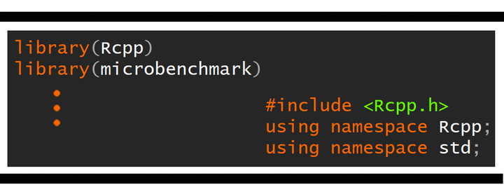
We are going to look at a concrete example of optimizing a function using Rcpp, and calling that function within R. We will need the library Rcpp, and we will be comparing execution times using the library microbenchmark. Both of these libraries can be installed easily:
install.packages("Rcpp")
install.packages("microbenchmark")
And then loaded in R:
library(Rcpp)
library(microbenchmark)
Example
This example is adapted from the application of filling a transition probability matrix (such as is typical when working with hidden Markov models).
Consider that we need to fill a matrix with calculated values. This is an issue that comes up all the time, and has many solutions. A few potential solutions for this problem include using the function outer(), looping over matrix elements with for loops, calculating row-wise or column-wise using the apply() function, etc. The various solutions each have their own computational efficiencies, with some being significantly faster than others. For demonstration we will use nested for loops in the R implementation.
For loops in R?
Typically, it is recommended to avoid using for loops in R when speed or efficiency are required. For loops are often slower than other (vectorized) solutions. However they are also the easiest method to learn for new programmers coming to R from other languages such as C++, where for loops can be very efficient.
R Implementation
The function we will be optimizing takes exactly one parameter, the size of the square matrix we will be filling with values.
func_forloop <- function(n) {
  M = matrix(0, nrow=n, ncol=n)
  for(row in 1:n) {
    for(col in 1:n) {
      for(m in 0:min(row,col)) {
        M[row,col] = M[row,col] +
          dpois(x = col-1-m, lambda = 1) *
          dbinom(x = m, size = row-1, prob = 0.75)
      }
    }
  }
  return(M)
}
We can calculate this matrix for any value of n, let’s try 3:
func_forloop(3)## [,1] [,2] [,3]
## [1,] 0.36787944 0.3678794 0.1839397
## [2,] 0.09196986 0.3678794 0.3218945
## [3,] 0.02299247 0.1609473 0.3563832So, how fast is this function?
bm = microbenchmark(func_forloop(10),
                    func_forloop(30),
                    func_forloop(50),
                    unit = "s")
print(bm, unit = "ms")
## Unit: milliseconds
## expr min lq mean median uq max neval
## func_forloop(10) 0.7996 0.85105 0.918849 0.8637 0.92460 2.0313 100
## func_forloop(30) 17.4439 18.72055 19.548081 19.3164 20.14695 24.6157 100
## func_forloop(50) 79.8493 83.20825 86.787526 85.9114 88.69220 108.6536 100As you can see, the function does not scale well as n increases (both dimensions of the matrix increase, and the upper bound of summation for m increase as n increases). Thus computing time can quickly grow out of hand for large n. Let’s see how we can implement this in C++ using Rcpp.
Rcpp Implementation
In a separate file (I will name the file my_func.cpp), we will have this implementation:
#include <Rcpp.h>
using namespace Rcpp;
using namespace std;

// [[Rcpp::export]]
NumericMatrix func_Rcpp(int x) {
  // NumericMatrix() is the Rcpp analogue to R's matrix()
  NumericMatrix M = NumericMatrix(x);

  // In C++ indexing starts at zero, not one
  for(int row = 0; row < x; row++) {
    for(int col = 0; col < x; col++) {
      for(int m = 0; m <= min(row,col); m++) {
        // C++ allows: "a += b" as shorthand for "a = a + b"
        M(row,col) += R::dpois(col-m, 1, false) *
          R::dbinom(m, row, 0.75, false);
      }
    }
  }

  return M;
}
We can then use the function in R after sourcing it with Rcpp:
Rcpp::sourceCpp("my_func.cpp")We can see that the function returns the same matrix as the R implementation:
func_Rcpp(3)## [,1] [,2] [,3]
## [1,] 0.36787944 0.3678794 0.1839397
## [2,] 0.09196986 0.3678794 0.3218945
## [3,] 0.02299247 0.1609473 0.3563832all.equal(func_forloop(3), func_Rcpp(3))## [1] TRUEAnd we can compare the computation times with the R implementation:
bm = microbenchmark(func_forloop(50),
                    func_Rcpp(50),
                    unit = "s")
print(bm, unit = "ms")
## Unit: milliseconds
## expr min lq mean median uq max neval
## func_forloop(50) 80.7933 85.1356 88.76877 87.81295 90.86310 126.9279 100
## func_Rcpp(50) 11.1477 11.2432 11.34730 11.28715 11.39125 12.3793 100The timings show that there is no contest, the for loop implementation in C++ is significantly faster. However, I would be remiss if I left you with the impression that this is the only way to speed up the code. This is meant as an example of implementing code using Rcpp, and calling that code from within R. Next I will show you a faster way of calculating this particular problem.
Convolution
The biggest bottleneck in this calculation is the summation over m. However, we are summing over the product of two functions, with one function input increasing and the other decreasing. In our case, this means we have a discrete convolution. It is well known that due to the existance of the Fast Fourier Transform, convolution can be calculated extremely quickly. Base R implements this fast convolution with the function convolve().
Using this fast convolution, the function looks like this:
func_convolution <- function(n) {
  M = matrix(0, nrow=n, ncol=n)
  for(row in 1:n) {
      M[row,] = convolve(dbinom(x = 0:n, size = row-1, prob = 0.75),
                         dpois(x = n:0, lambda = 1),
                         type = "open")[1:n]
  }
  return(M)
}func_convolution(3)## [,1] [,2] [,3]
## [1,] 0.36787944 0.3678794 0.1839397
## [2,] 0.09196986 0.3678794 0.3218945
## [3,] 0.02299247 0.1609473 0.3563832all.equal(func_forloop(3), func_Rcpp(3), func_convolution(3))## [1] TRUEbm = microbenchmark(func_forloop(50),
func_Rcpp(50),
func_convolution(50),
unit = "s")
print(bm, unit = "ms")## Unit: milliseconds
## expr min lq mean median uq max
## func_forloop(50) 80.1737 82.31445 88.196659 83.88585 88.52630 143.7698
## func_Rcpp(50) 11.1441 11.22830 11.513228 11.25875 11.41995 17.5220
## func_convolution(50) 1.9157 2.07120 2.140127 2.11385 2.19880 3.2247
## neval
## 100
## 100
## 100So, the convolution method performs even better than the Rcpp implementation. What is the drawback? Well, the convolution method is extremely fast, but only very narrowly applicable.
Vectorized
We can also vectorize to remove the need for the for loop entirely:
func_vectorized <- function(n) {
  M = matrix(0, nrow=n, ncol=n)

  M = t(sapply(X = 1:n, FUN = function(X) {
    convolve(dbinom(x = 0:n, size = X-1, prob = 0.75),
                         dpois(x = n:0, lambda = 1),
                         type = "open")[1:n]
  }))

  return(M)
}
func_vectorized(3)
## [,1] [,2] [,3]
## [1,] 0.36787944 0.3678794 0.1839397
## [2,] 0.09196986 0.3678794 0.3218945
## [3,] 0.02299247 0.1609473 0.3563832bm = microbenchmark(func_convolution(300),
func_vectorized(300),
unit = "s")
print(bm, unit = "ms")## Unit: milliseconds
## expr min lq mean median uq max
## func_convolution(300) 185.9818 189.2231 202.6476 191.6806 193.8182 340.8995
## func_vectorized(300) 187.5353 190.1851 200.1388 192.5210 194.6368 280.7497
## neval
## 100
## 100However, you can see that in this case, the for loop is essentially the same speed as the vectorized solution.
Conclusions
Rcpp can be applied to many more types of problems to optimize your R code, but you should always be aware that small computational tricks such as convolution can vastly improve the performance of your code. Knowing how to take advantage of C++ to speed up portions of your code can save tremendous amounts of time for complicated or long-running programs. The goal should be to program in R, use code profiling to find bottlenecks, and optimize those bottlenecks (either using Rcpp, or refactoring the code, or using mathematical tricks).